Takes a formula and a dataframe as input, conducts an analysis of variance prints the results (AOV summary table, table of overall model information and table of means) then uses ggplot2 to plot an interaction graph (line or bar) . Also uses Brown-Forsythe test for homogeneity of variance. Users can also choose to save the plot out as a png file.
Plot2WayANOVA(formula,
               dataframe = NULL,
               confidence=.95,
               plottype = "line",
               errorbar.display = "CI",
               xlab = NULL,
               ylab = NULL,
               title = NULL,
               subtitle = NULL,
               interact.line.size = 2,
               ci.line.size = 1,
               mean.label = FALSE,
               mean.ci = TRUE,
               mean.size = 4,
               mean.shape = 23,
               mean.color = "darkred",
               mean.label.size = 3,
               mean.label.color = "black",
               offset.style = "none",
               overlay.type = NULL,
               posthoc.method = "scheffe",
               show.dots = FALSE,
               PlotSave = FALSE,
               ggtheme = ggplot2::theme_bw(),
               package = "RColorBrewer",
               palette = "Dark2",
               ggplot.component = NULL)
Arguments
| formula | a formula with a numeric dependent (outcome) variable,
and two independent (predictor) variables e.g. |
|---|---|
| dataframe | a dataframe or an object that can be coerced to a dataframe |
| confidence | what confidence level for confidence intervals |
| plottype | bar or line (quoted) |
| errorbar.display | default "CI" (confidence interval), which type of
errorbar should be displayed around the mean point? Other options
include "SEM" (standard error of the mean) and "SD" (standard dev).
"none" removes it entirely much like |
| xlab, ylab | Labels for `x` and `y` axis variables. If `NULL` (default), variable names for `x` and `y` will be used. |
| title | The text for the plot title. A generic default is provided. |
| subtitle | The text for the plot subtitle. If `NULL` (default), key model information is provided as a subtitle. |
| interact.line.size | Line size for the line connecting the group means (Default: `2`). |
| ci.line.size | Line size for the confidence interval bracketing the group means (Default: `1`). |
| mean.label | Logical that decides whether the value of the group mean is to be displayed (Default: `FALSE`). |
| mean.ci | Logical that decides whether the confidence interval for group means is to be displayed (Default: `TRUE`). |
| mean.size | Point size for the data point corresponding to mean (Default: `4`). |
| mean.shape | Shape of the plot symbol for the mean (Default: `23` which is a diamond). |
| mean.color | Color for the data point corresponding to mean (Default: `"darkred"`). |
| mean.label.size, mean.label.color | Aesthetics for the label displaying mean. Defaults: `3`, `"black"`, respectively. |
| offset.style | A character string (e.g., `"wide"` or `"narrow"`, or `"none"`) which controls whether items are offset from the centerline for clarity. Useful when you want to add individual datapoints or confdence interval lines overlap. (Default: `"none"`). |
| overlay.type | A character string (e.g., `"box"` or `"violin"`), if you wish to overlay that information on factor1 |
| posthoc.method | A character string, one of "hsd", "bonf", "lsd", "scheffe", "newmankeuls", defining the method for the pairwise comparisons. (Default: `"scheffe"`). |
| show.dots | Logical that decides whether the individual data points are displayed (Default: `FALSE`). |
| PlotSave | a logical indicating whether the user wants to save the plot as a png file |
| ggtheme | A function, ggplot2 theme name. Default value is ggplot2::theme_bw(). Any of the ggplot2 themes, or themes from extension packages are allowed (e.g., hrbrthemes::theme_ipsum(), etc.). |
| package | Name of package from which the palette is desired as string or symbol. |
| palette | Name of palette as string or symbol. |
| ggplot.component | A ggplot component to be added to the plot prepared. The default is NULL. The argument should be entered as a function. for example to change the size and color of the x axis text you use: `ggplot.component = theme(axis.text.x = element_text(size=13, color="darkred"))` depending on what theme is in use the ggplot component might not work as expected. |
Value
A list with 5 elements which is returned invisibly. These items
are always sent to the console for display but for user convenience
the function also returns a named list with the following items
in case the user desires to save them or further process them -
$ANOVATable, $ModelSummary, $MeansTable,
$PosthocTable, $BFTest, and $SWTest.
The plot is always sent to the default plot device
Details
Details about how the function works in order of steps taken.
Some basic error checking to ensure a valid formula and dataframe. Only accepts fully *crossed* formula to check for interaction term
Ensure the dependent (outcome) variable is numeric and that the two independent (predictor) variables are or can be coerced to factors -- user warned on the console
Remove missing cases -- user warned on the console
Calculate a summarized table of means, sds, standard errors of the means, confidence intervals, and group sizes.
Use
aovfunction to execute an Analysis of Variance (ANOVA)Use
sjstats::anova_statsto calculate eta squared and omega squared values per factor. If the design is unbalanced warn the user and use Type II sums of squaresProduce a standard ANOVA table with additional columns
Use the
PostHocTestfor producing a table of post hoc comparisons for all effects that were significantTesting Homogeneity of Variance assumption with Brown-Forsythe test
Use the
PostHocTestfor conducting post hoc tests for effects that were significantUse the
shapiro.testfor testing normality assumption with Shapiro-WilkUse
ggplot2to plot an interaction plot of the type the user specified.
The defaults are deliberately constructed to emphasize the nature of the interaction rather than focusing on distributions. So while a violin plot of the first factor by level is displayed along with dots for individual data points shaded by the second factor, the emphasis is on the interaction lines.
References
: ANOVA: Delacre, Leys, Mora, & Lakens, *PsyArXiv*, 2018
See also
Author
Chuck Powell
Examples
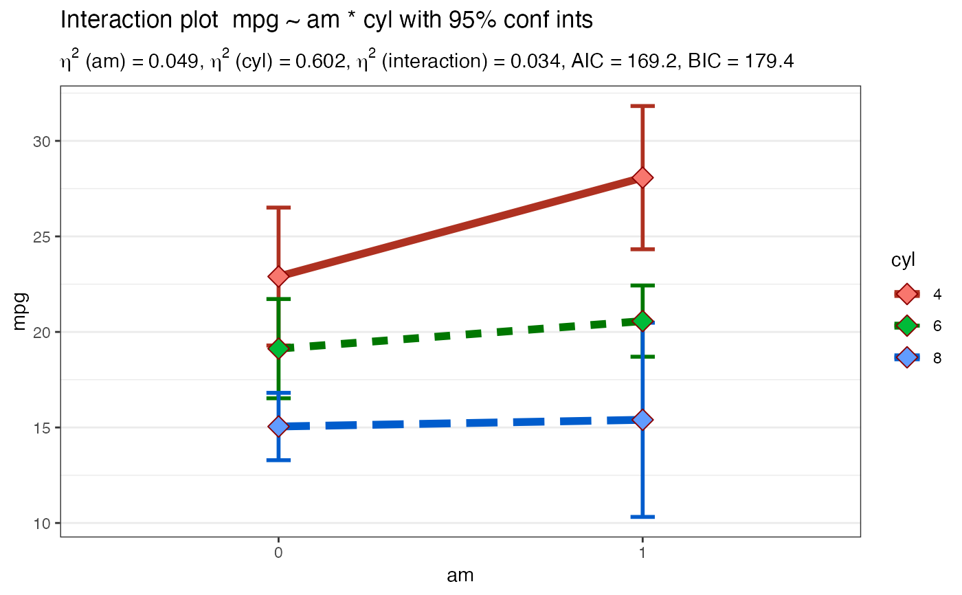
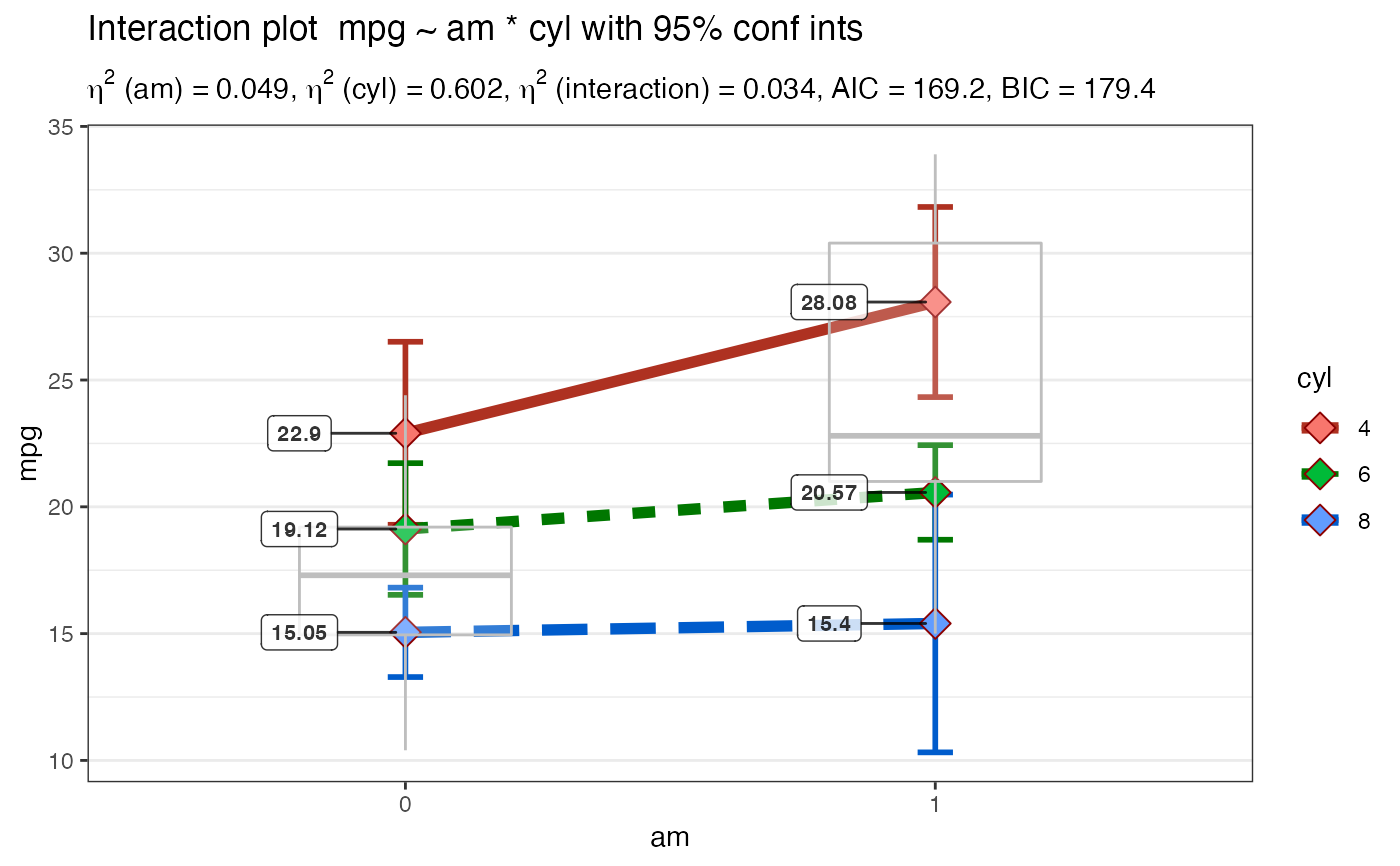
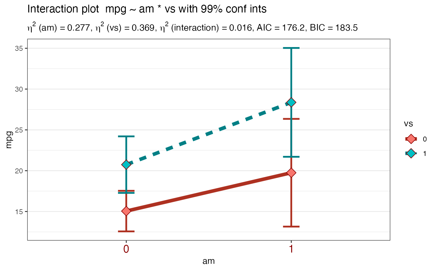
Plot2WayANOVA(mpg ~ am * cyl, mtcars, plottype = "line")#> #>#> #>#> #> #>#> # A tibble: 6 x 3 #> am cyl count #> <fct> <fct> <dbl> #> 1 0 4 3 #> 2 0 6 4 #> 3 0 8 12 #> 4 1 4 8 #> 5 1 6 3 #> 6 1 8 2#> #> #> #> #> #>#> term sumsq meansq df statistic p.value etasq partial.etasq #> am am 36.767 36.767 1 3.999 0.056 0.049 0.133 #> cyl cyl 456.401 228.200 2 24.819 0.000 0.602 0.656 #> am:cyl am:cyl 25.437 12.718 2 1.383 0.269 0.034 0.096 #> ...4 Residuals 239.059 9.195 26 NA NA NA NA #> omegasq partial.omegasq epsilonsq cohens.f power #> am 0.036 0.086 0.036 0.392 0.515 #> cyl 0.571 0.598 0.578 1.382 1.000 #> am:cyl 0.009 0.023 0.009 0.326 0.298 #> ...4 NA NA NA NA NA#> #>#> # A tibble: 6 x 15 #> # Groups: am [2] #> am cyl TheMean TheSD TheSEM CIMuliplier LowerBoundCI UpperBoundCI #> <fct> <fct> <dbl> <dbl> <dbl> <dbl> <dbl> <dbl> #> 1 0 4 22.9 1.45 0.839 4.30 19.3 26.5 #> 2 0 6 19.1 1.63 0.816 3.18 16.5 21.7 #> 3 0 8 15.0 2.77 0.801 2.20 13.3 16.8 #> 4 1 4 28.1 4.48 1.59 2.36 24.3 31.8 #> 5 1 6 20.6 0.751 0.433 4.30 18.7 22.4 #> 6 1 8 15.4 0.566 0.4 12.7 10.3 20.5 #> # … with 7 more variables: LowerBoundSEM <dbl>, UpperBoundSEM <dbl>, #> # LowerBoundSD <dbl>, UpperBoundSD <dbl>, N <int>, LowerBound <dbl>, #> # UpperBound <dbl>#> #>#> #> Posthoc multiple comparisons of means: Scheffe Test #> 95% family-wise confidence level #> #> $cyl #> diff lwr.ci upr.ci pval #> 6-4 -4.756706 -10.029278 0.5158655 0.09684 . #> 8-4 -7.329581 -11.723391 -2.9357710 0.00024 *** #> 8-6 -2.572874 -7.620978 2.4752288 0.64828 #> #> --- #> Signif. codes: 0 '***' 0.001 '**' 0.01 '*' 0.05 '.' 0.1 ' ' 1 #>#> #>#>#> Brown-Forsythe Test for Homogeneity of Variance using median #> Df F value Pr(>F) #> group 5 2.736 0.04086 * #> 26 #> --- #> Signif. codes: 0 ‘***’ 0.001 ‘**’ 0.01 ‘*’ 0.05 ‘.’ 0.1 ‘ ’ 1#> #>#> #> Shapiro-Wilk normality test #> #> data: MyAOV_residuals #> W = 0.96277, p-value = 0.3263 #>#> #>#> # A tibble: 4 x 4 #> model bf support margin_of_error #> <chr> <dbl> <chr> <dbl> #> 1 am + cyl 4228908. " data support is extreme" 0.0124 #> 2 am + cyl + am:cyl 3083523. " data support is extreme" 0.0224 #> 3 cyl 2274206. " data support is extreme" 0.0000000127 #> 4 am 86.6 " data support is very strong" 0.000000217#> #>Plot2WayANOVA(mpg ~ am * cyl, mtcars, plottype = "line", overlay.type = "box", mean.label = TRUE )#> #>#> #>#> #> #>#> # A tibble: 6 x 3 #> am cyl count #> <fct> <fct> <dbl> #> 1 0 4 3 #> 2 0 6 4 #> 3 0 8 12 #> 4 1 4 8 #> 5 1 6 3 #> 6 1 8 2#> #> #> #> #> #>#> term sumsq meansq df statistic p.value etasq partial.etasq #> am am 36.767 36.767 1 3.999 0.056 0.049 0.133 #> cyl cyl 456.401 228.200 2 24.819 0.000 0.602 0.656 #> am:cyl am:cyl 25.437 12.718 2 1.383 0.269 0.034 0.096 #> ...4 Residuals 239.059 9.195 26 NA NA NA NA #> omegasq partial.omegasq epsilonsq cohens.f power #> am 0.036 0.086 0.036 0.392 0.515 #> cyl 0.571 0.598 0.578 1.382 1.000 #> am:cyl 0.009 0.023 0.009 0.326 0.298 #> ...4 NA NA NA NA NA#> #>#> # A tibble: 6 x 15 #> # Groups: am [2] #> am cyl TheMean TheSD TheSEM CIMuliplier LowerBoundCI UpperBoundCI #> <fct> <fct> <dbl> <dbl> <dbl> <dbl> <dbl> <dbl> #> 1 0 4 22.9 1.45 0.839 4.30 19.3 26.5 #> 2 0 6 19.1 1.63 0.816 3.18 16.5 21.7 #> 3 0 8 15.0 2.77 0.801 2.20 13.3 16.8 #> 4 1 4 28.1 4.48 1.59 2.36 24.3 31.8 #> 5 1 6 20.6 0.751 0.433 4.30 18.7 22.4 #> 6 1 8 15.4 0.566 0.4 12.7 10.3 20.5 #> # … with 7 more variables: LowerBoundSEM <dbl>, UpperBoundSEM <dbl>, #> # LowerBoundSD <dbl>, UpperBoundSD <dbl>, N <int>, LowerBound <dbl>, #> # UpperBound <dbl>#> #>#> #> Posthoc multiple comparisons of means: Scheffe Test #> 95% family-wise confidence level #> #> $cyl #> diff lwr.ci upr.ci pval #> 6-4 -4.756706 -10.029278 0.5158655 0.09684 . #> 8-4 -7.329581 -11.723391 -2.9357710 0.00024 *** #> 8-6 -2.572874 -7.620978 2.4752288 0.64828 #> #> --- #> Signif. codes: 0 '***' 0.001 '**' 0.01 '*' 0.05 '.' 0.1 ' ' 1 #>#> #>#>#> Brown-Forsythe Test for Homogeneity of Variance using median #> Df F value Pr(>F) #> group 5 2.736 0.04086 * #> 26 #> --- #> Signif. codes: 0 ‘***’ 0.001 ‘**’ 0.01 ‘*’ 0.05 ‘.’ 0.1 ‘ ’ 1#> #>#> #> Shapiro-Wilk normality test #> #> data: MyAOV_residuals #> W = 0.96277, p-value = 0.3263 #>#> #>#> # A tibble: 4 x 4 #> model bf support margin_of_error #> <chr> <dbl> <chr> <dbl> #> 1 am + cyl 4187558. " data support is extreme" 0.0106 #> 2 am + cyl + am:cyl 3113288. " data support is extreme" 0.0263 #> 3 cyl 2274206. " data support is extreme" 0.0000000127 #> 4 am 86.6 " data support is very strong" 0.000000217#> #>library(ggplot2) Plot2WayANOVA(mpg ~ am * vs, mtcars, confidence = .99, ggplot.component = theme(axis.text.x = element_text(size=13, color="darkred")))#> #>#> #>#> #> #> #> #> #>#> term sumsq meansq df statistic p.value etasq partial.etasq #> am am 276.033 276.033 1 22.902 0.000 0.277 0.450 #> vs vs 367.411 367.411 1 30.484 0.000 0.369 0.521 #> am:vs am:vs 16.010 16.010 1 1.328 0.259 0.016 0.045 #> ...4 Residuals 337.476 12.053 28 NA NA NA NA #> omegasq partial.omegasq epsilonsq cohens.f power #> am 0.262 0.406 0.265 0.904 0.998 #> vs 0.352 0.480 0.356 1.043 1.000 #> am:vs 0.004 0.010 0.004 0.218 0.211 #> ...4 NA NA NA NA NA#> #>#> # A tibble: 4 x 15 #> # Groups: am [2] #> am vs TheMean TheSD TheSEM CIMuliplier LowerBoundCI UpperBoundCI #> <fct> <fct> <dbl> <dbl> <dbl> <dbl> <dbl> <dbl> #> 1 0 0 15.0 2.77 0.801 3.11 12.6 17.5 #> 2 0 1 20.7 2.47 0.934 3.71 17.3 24.2 #> 3 1 0 19.8 4.01 1.64 4.03 13.2 26.3 #> 4 1 1 28.4 4.76 1.80 3.71 21.7 35.0 #> # … with 7 more variables: LowerBoundSEM <dbl>, UpperBoundSEM <dbl>, #> # LowerBoundSD <dbl>, UpperBoundSD <dbl>, N <int>, LowerBound <dbl>, #> # UpperBound <dbl>#> #>#> #> Posthoc multiple comparisons of means: Scheffe Test #> 99% family-wise confidence level #> #> $am #> diff lwr.ci upr.ci pval #> 1-0 7.244939 2.619029 11.87085 5.3e-05 *** #> #> $vs #> diff lwr.ci upr.ci pval #> 1-0 6.732986 2.153198 11.31277 0.00013 *** #> #> --- #> Signif. codes: 0 '***' 0.001 '**' 0.01 '*' 0.05 '.' 0.1 ' ' 1 #>#> #>#> Brown-Forsythe Test for Homogeneity of Variance using median #> Df F value Pr(>F) #> group 3 0.8809 0.4629 #> 28#> #>#> #> Shapiro-Wilk normality test #> #> data: MyAOV_residuals #> W = 0.97845, p-value = 0.7535 #>#> #>#> # A tibble: 4 x 4 #> model bf support margin_of_error #> <chr> <dbl> <chr> <dbl> #> 1 am + vs 200567. " data support is extreme" 0.0153 #> 2 am + vs + am:vs 123044. " data support is extreme" 0.0140 #> 3 vs 529. " data support is extreme" 0.00000000901 #> 4 am 86.6 " data support is very strong" 0.000000217#> #>