Introducing the CGPfunctions package -- March 22, 2018
Tagged as: [Overview
This package includes functions that I find useful for teaching statistics as well as actually practicing the art. They typically are not “new” methods but rather wrappers around either base R or other packages and concepts I’m trying to master. Currently contains:
Plot2WayANOVAwhich as the name implies conducts a 2 way ANOVA and plots the results usingggplot2newetawhich is a helper function that appends the results of a Type II eta squared calculation onto a classic ANOVA tableModewhich finds the modal value in a vector of dataSeeDistwhich wraps around ggplot2 to provide visualizations of univariate data.OurConfis a simulation function that helps you learn about confidence intervals
Installation
# Install from CRAN
install.packages("CGPfunctions")

# Highly recommended since it is under rapid development right now
# Or the development version from GitHub
# install.packages("devtools")
devtools::install_github("ibecav/CGPfunctions")
Usage
library(CGPfunctions) will load the package which contains 5
functions:
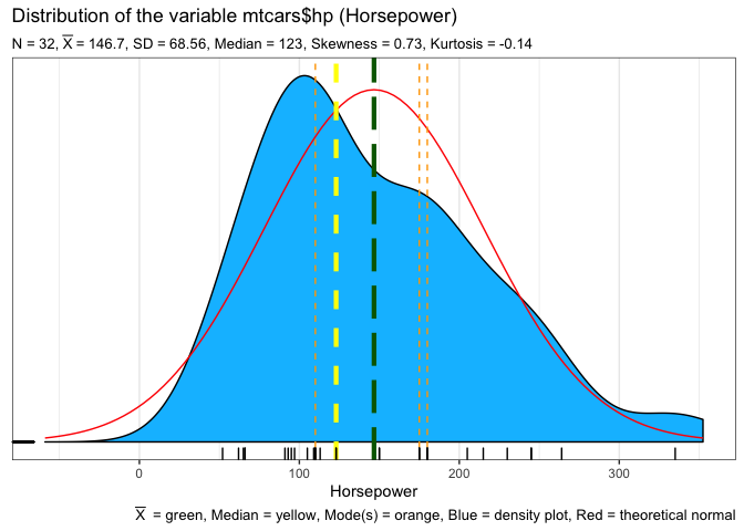
SeeDist will give you some plots of the distribution of a variable
using ggplot2
library(CGPfunctions)
SeeDist(mtcars$hp,whatvar="Horsepower",whatplots="d")

#>    Min. 1st Qu.  Median    Mean 3rd Qu.    Max.
#>    52.0    96.5   123.0   146.7   180.0   335.0
Mode is a helper function that simply returns one or more modal values
Mode(mtcars$hp)
#> [1] 110 175 180
neweta is a helper function which returns a tibble containing AOV
output similar to summary(aov(MyAOV)) but with eta squared computed and
appended as an additional column
MyAOV <- aov(mpg~am*cyl, mtcars)
neweta(MyAOV)
#> # A tibble: 4 x 8
#>   Source       Df `Sum Sq` `Mean Sq` `F value`       p sigstars `eta sq`
#>   <fct>     <int>    <dbl>     <dbl>     <dbl>   <dbl> <chr>       <dbl>
#> 1 am            1     37.0     37.0       4.30  0.0480 *          0.0330
#> 2 cyl           1    450.     450.       52.0   0.     ***        0.399
#> 3 am:cyl        1     29.4     29.4       3.40  0.0760 .          0.0260
#> 4 Residuals    28    242.       8.64     NA    NA      <NA>       0.215
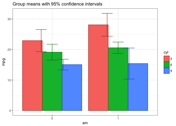
The Plot2WayANOVA function conducts a classic analysis using existing
R functions and packages in a sane and defensible manner not necessarily
in the one and only manner.
Plot2WayANOVA(mpg~am*cyl, mtcars)
#>
#> Converting am to a factor --- check your results
#>
#> Converting cyl to a factor --- check your results
#>
#> You have an unbalanced design. Using Type II sum of squares, eta squared may not sum to 1.0
#> # A tibble: 4 x 8
#>   Source       Df `Sum Sq` `Mean Sq` `F value`       p sigstars `eta sq`
#>   <fct>     <int>    <dbl>     <dbl>     <dbl>   <dbl> <chr>       <dbl>
#> 1 am            1     36.8     36.8       4.00  0.0560 .          0.0330
#> 2 cyl           2    456.     228.       24.8   0.     ***        0.405
#> 3 am:cyl        2     25.4     12.7       1.40  0.269  ""         0.0230
#> 4 Residuals    26    239.       9.19     NA    NA      <NA>       0.212
#>
#> Table of group means
#> # A tibble: 6 x 9
#> # Groups:   am [2]
#>   am    cyl   TheMean TheSD TheSEM CIMuliplier LowerBound UpperBound     N
#>   <fct> <fct>   <dbl> <dbl>  <dbl>       <dbl>      <dbl>      <dbl> <int>
#> 1 0     4        22.9 1.45   0.839        4.30       19.3       26.5     3
#> 2 0     6        19.1 1.63   0.816        3.18       16.5       21.7     4
#> 3 0     8        15.0 2.77   0.801        2.20       13.3       16.8    12
#> 4 1     4        28.1 4.48   1.59         2.36       24.3       31.8     8
#> 5 1     6        20.6 0.751  0.433        4.30       18.7       22.4     3
#> 6 1     8        15.4 0.566  0.400       12.7        10.3       20.5     2
#>
#> Testing Homogeneity of Variance with Brown-Forsythe
#>    *** Possible violation of the assumption ***
#> Levene's Test for Homogeneity of Variance (center = median)
#>       Df F value  Pr(>F)
#> group  5   2.736 0.04086 *
#>       26
#> ---
#> Signif. codes:  0 '***' 0.001 '**' 0.01 '*' 0.05 '.' 0.1 ' ' 1
#>
#> Testing Normality Assumption with Shapiro-Wilk
#>
#>  Shapiro-Wilk normality test
#>
#> data:  MyAOV_residuals
#> W = 0.96277, p-value = 0.3263
#>
#> Interaction graph plotted...

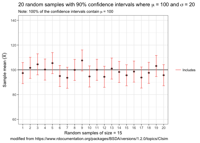
OurConf is a simulation function that helps you learn about confidence
intervals
OurConf(samples = 20, n = 15, mu = 100, sigma = 20, conf.level = 0.90)

#> 100 % of the confidence intervals contain Mu = 100 .
Credits
Many thanks to Dani Navarro and the book > (Learning Statistics with
R)
whose etaSquared function was the genesis of neweta.
“He who gives up safety for speed deserves neither.” (via)
A shoutout to some other packages I find essential.
- stringr, for strings.
- lubridate, for date/times.
- forcats, for factors.
- haven, for SPSS, SAS and Stata files.
- readxl, for
.xlsand.xlsxfiles. - modelr, for modelling within a pipeline
- broom, for turning models into tidy data
- ggplot2, for data visualisation.
- dplyr, for data manipulation.
- tidyr, for data tidying.
- readr, for data import.
- purrr, for functional programming.
- tibble, for tibbles, a modern re-imagining of data frames.
Leaving Feedback
If you like CGPfunctions, please consider leaving feedback here.
Contributing
Contributions in the form of feedback, comments, code, and bug reports are most welcome. How to contribute:
- Issues, bug reports, and wish lists: File a GitHub issue.
- Contact the maintainer ibecav at gmail.com by email.
License

This work (blogpost) is licensed under a
Creative
Commons Attribution-ShareAlike 4.0 International License.