CHAID and R -- When you need explanation – May 15, 2018
Tagged as: [A modern data scientist using R has access to an almost bewildering number of tools, libraries and algorithms to analyze the data. In my next two posts I’m going to focus on an in depth visit with CHAID (Chi-square automatic interaction detection). The title should give you a hint for why I think CHAID is a good “tool” for your analytical toolbox. There are lots of tools that can help you predict or classify but CHAID is especially good at helping you explain to any audience how the model arrives at it’s prediction or classification. It’s also incredibly robust from a statistical perspective, making almost no assumptions about your data for distribution or normality. I’ll try and elaborate on that as we work the example.
You can get a very brief summary of CHAID from wikipedia and mentions of it scattered about in places like Analytics Vidhya or Data Flair. If you prefer a more scholarly bent the original article can be found in places like JSTOR. As the name implies it is fundamentally based on the venerable Chi-square test – and while not the most powerful (in terms of detecting the smallest possible differences) or the fastest, it really is easy to manage and more importantly to tell the story after using it.
Compared to some other techniques it’s also quite simple to use, as I
hope you’ll agree, by the end of these posts. To showcase it we’re going
to be using a dataset that comes to us from the IBM Watson
Project
and comes packaged with the rsample library. It’s a very practical and
understandable dataset. A great use case for a tree based algorithm.
Imagine yourself in a fictional company faced with the task of trying to
figure out which employees you are going to “lose” a.k.a. attrition or
turnover. There’s a steep cost involved in keeping good employees and
training and on-boarding can be expensive. Being able to predict
attrition even a little bit better would save you lots of money and make
the company better, especially if you can understand exactly what you
have to “watch out” for that might indicate the person is a high risk to
leave.
Setup and library loading
If you’ve never used CHAID before you may also not have partykit.
CHAID isn’t on CRAN but I have commented out the install command
below. You’ll also get a variety of messages, none of which is relevant
to this example so I’ve suppressed them.
# install.packages("partykit")
# install.packages("CHAID", repos="http://R-Forge.R-project.org")
require(rsample) # for dataset and splitting also loads broom and tidyr
require(dplyr)
require(ggplot2)
theme_set(theme_bw()) # set theme
require(CHAID)
require(purrr)
require(caret)
Predicting attrition in a fictional company
Let’s load up the attrition dataset and take a look at the variables
we have.
# data(attrition)
str(attrition)
## 'data.frame':    1470 obs. of  31 variables:
##  $ Age                     : int  41 49 37 33 27 32 59 30 38 36 ...
##  $ Attrition               : Factor w/ 2 levels "No","Yes": 2 1 2 1 1 1 1 1 1 1 ...
##  $ BusinessTravel          : Factor w/ 3 levels "Non-Travel","Travel_Frequently",..: 3 2 3 2 3 2 3 3 2 3 ...
##  $ DailyRate               : int  1102 279 1373 1392 591 1005 1324 1358 216 1299 ...
##  $ Department              : Factor w/ 3 levels "Human_Resources",..: 3 2 2 2 2 2 2 2 2 2 ...
##  $ DistanceFromHome        : int  1 8 2 3 2 2 3 24 23 27 ...
##  $ Education               : Ord.factor w/ 5 levels "Below_College"<..: 2 1 2 4 1 2 3 1 3 3 ...
##  $ EducationField          : Factor w/ 6 levels "Human_Resources",..: 2 2 5 2 4 2 4 2 2 4 ...
##  $ EnvironmentSatisfaction : Ord.factor w/ 4 levels "Low"<"Medium"<..: 2 3 4 4 1 4 3 4 4 3 ...
##  $ Gender                  : Factor w/ 2 levels "Female","Male": 1 2 2 1 2 2 1 2 2 2 ...
##  $ HourlyRate              : int  94 61 92 56 40 79 81 67 44 94 ...
##  $ JobInvolvement          : Ord.factor w/ 4 levels "Low"<"Medium"<..: 3 2 2 3 3 3 4 3 2 3 ...
##  $ JobLevel                : int  2 2 1 1 1 1 1 1 3 2 ...
##  $ JobRole                 : Factor w/ 9 levels "Healthcare_Representative",..: 8 7 3 7 3 3 3 3 5 1 ...
##  $ JobSatisfaction         : Ord.factor w/ 4 levels "Low"<"Medium"<..: 4 2 3 3 2 4 1 3 3 3 ...
##  $ MaritalStatus           : Factor w/ 3 levels "Divorced","Married",..: 3 2 3 2 2 3 2 1 3 2 ...
##  $ MonthlyIncome           : int  5993 5130 2090 2909 3468 3068 2670 2693 9526 5237 ...
##  $ MonthlyRate             : int  19479 24907 2396 23159 16632 11864 9964 13335 8787 16577 ...
##  $ NumCompaniesWorked      : int  8 1 6 1 9 0 4 1 0 6 ...
##  $ OverTime                : Factor w/ 2 levels "No","Yes": 2 1 2 2 1 1 2 1 1 1 ...
##  $ PercentSalaryHike       : int  11 23 15 11 12 13 20 22 21 13 ...
##  $ PerformanceRating       : Ord.factor w/ 4 levels "Low"<"Good"<"Excellent"<..: 3 4 3 3 3 3 4 4 4 3 ...
##  $ RelationshipSatisfaction: Ord.factor w/ 4 levels "Low"<"Medium"<..: 1 4 2 3 4 3 1 2 2 2 ...
##  $ StockOptionLevel        : int  0 1 0 0 1 0 3 1 0 2 ...
##  $ TotalWorkingYears       : int  8 10 7 8 6 8 12 1 10 17 ...
##  $ TrainingTimesLastYear   : int  0 3 3 3 3 2 3 2 2 3 ...
##  $ WorkLifeBalance         : Ord.factor w/ 4 levels "Bad"<"Good"<"Better"<..: 1 3 3 3 3 2 2 3 3 2 ...
##  $ YearsAtCompany          : int  6 10 0 8 2 7 1 1 9 7 ...
##  $ YearsInCurrentRole      : int  4 7 0 7 2 7 0 0 7 7 ...
##  $ YearsSinceLastPromotion : int  0 1 0 3 2 3 0 0 1 7 ...
##  $ YearsWithCurrManager    : int  5 7 0 0 2 6 0 0 8 7 ...
Okay we have data on 1,470 employees. We have 30 potential predictor or
independent variables and the all important attrition variable which
gives us a yes or no answer to the question of whether or not the
employee left. We’re to build the most accurate predictive model we can
that is also simple (parsimonious) and explainable. The predictors we
have seem to be the sorts of data we might have on hand in our HR files
and thank goodness are labelled in a way that makes them pretty self
explanatory.
The CHAID library in R requires that any variables that we enter as
predictors be either nominal or ordinal variables (see ?CHAID::chaid),
which in R speak means we have to get them in as either factor or
ordered factor. The str command shows we have a bunch of variables
which are of type integer. As it turns out moving from integer to
factor is simple in terms of code but has to be thoughtful for
substantive reasons. So let’s see how things breakdown.
attrition %>%
  select_if(is.factor) %>%
  ncol
## [1] 15
attrition %>%
  select_if(is.numeric) %>%
  ncol
## [1] 16
Hmmmm, 15 factors and 16 integers. Let’s explore further. Of the
variables that are integers how many of them have a small number of
values (a.k.a. levels) and can therefore be simply and easily converted
to true factors. We’ll use a dplyr pipe to see how many have 5 or
fewer levels and 10 or fewer levels.
attrition %>%
  select_if(function(col)
    length(unique(col)) <= 5 & is.integer(col)) %>%
  head
##   JobLevel StockOptionLevel
## 1        2                0
## 2        2                1
## 4        1                0
## 5        1                0
## 7        1                1
## 8        1                0
attrition %>%
  select_if(function(col)
    length(unique(col)) <= 10 & is.integer(col)) %>%
  head
##   JobLevel NumCompaniesWorked StockOptionLevel TrainingTimesLastYear
## 1        2                  8                0                     0
## 2        2                  1                1                     3
## 4        1                  6                0                     3
## 5        1                  1                0                     3
## 7        1                  9                1                     3
## 8        1                  0                0                     2
2 and 4 respectively. We can be pretty confident that converting these
from integer to factor won’t lose much information. Simple to run a
mutate operation across the 4 we have identified. Probably more
elegant though to make it a mutate_if. That way in the future we
decide we like 4 or 7 or 122 as our criteria for the change we only have
to change one number. The “if” variation is also less to type and less
likely to make a manual mistake.
attrition %>%
  mutate(
    JobLevel = factor(JobLevel),
    NumCompaniesWorked = factor(NumCompaniesWorked),
    StockOptionLevel = factor(StockOptionLevel),
    TrainingTimesLastYear = factor(TrainingTimesLastYear)
  ) %>%
  str
## 'data.frame':    1470 obs. of  31 variables:
##  $ Age                     : int  41 49 37 33 27 32 59 30 38 36 ...
##  $ Attrition               : Factor w/ 2 levels "No","Yes": 2 1 2 1 1 1 1 1 1 1 ...
##  $ BusinessTravel          : Factor w/ 3 levels "Non-Travel","Travel_Frequently",..: 3 2 3 2 3 2 3 3 2 3 ...
##  $ DailyRate               : int  1102 279 1373 1392 591 1005 1324 1358 216 1299 ...
##  $ Department              : Factor w/ 3 levels "Human_Resources",..: 3 2 2 2 2 2 2 2 2 2 ...
##  $ DistanceFromHome        : int  1 8 2 3 2 2 3 24 23 27 ...
##  $ Education               : Ord.factor w/ 5 levels "Below_College"<..: 2 1 2 4 1 2 3 1 3 3 ...
##  $ EducationField          : Factor w/ 6 levels "Human_Resources",..: 2 2 5 2 4 2 4 2 2 4 ...
##  $ EnvironmentSatisfaction : Ord.factor w/ 4 levels "Low"<"Medium"<..: 2 3 4 4 1 4 3 4 4 3 ...
##  $ Gender                  : Factor w/ 2 levels "Female","Male": 1 2 2 1 2 2 1 2 2 2 ...
##  $ HourlyRate              : int  94 61 92 56 40 79 81 67 44 94 ...
##  $ JobInvolvement          : Ord.factor w/ 4 levels "Low"<"Medium"<..: 3 2 2 3 3 3 4 3 2 3 ...
##  $ JobLevel                : Factor w/ 5 levels "1","2","3","4",..: 2 2 1 1 1 1 1 1 3 2 ...
##  $ JobRole                 : Factor w/ 9 levels "Healthcare_Representative",..: 8 7 3 7 3 3 3 3 5 1 ...
##  $ JobSatisfaction         : Ord.factor w/ 4 levels "Low"<"Medium"<..: 4 2 3 3 2 4 1 3 3 3 ...
##  $ MaritalStatus           : Factor w/ 3 levels "Divorced","Married",..: 3 2 3 2 2 3 2 1 3 2 ...
##  $ MonthlyIncome           : int  5993 5130 2090 2909 3468 3068 2670 2693 9526 5237 ...
##  $ MonthlyRate             : int  19479 24907 2396 23159 16632 11864 9964 13335 8787 16577 ...
##  $ NumCompaniesWorked      : Factor w/ 10 levels "0","1","2","3",..: 9 2 7 2 10 1 5 2 1 7 ...
##  $ OverTime                : Factor w/ 2 levels "No","Yes": 2 1 2 2 1 1 2 1 1 1 ...
##  $ PercentSalaryHike       : int  11 23 15 11 12 13 20 22 21 13 ...
##  $ PerformanceRating       : Ord.factor w/ 4 levels "Low"<"Good"<"Excellent"<..: 3 4 3 3 3 3 4 4 4 3 ...
##  $ RelationshipSatisfaction: Ord.factor w/ 4 levels "Low"<"Medium"<..: 1 4 2 3 4 3 1 2 2 2 ...
##  $ StockOptionLevel        : Factor w/ 4 levels "0","1","2","3": 1 2 1 1 2 1 4 2 1 3 ...
##  $ TotalWorkingYears       : int  8 10 7 8 6 8 12 1 10 17 ...
##  $ TrainingTimesLastYear   : Factor w/ 7 levels "0","1","2","3",..: 1 4 4 4 4 3 4 3 3 4 ...
##  $ WorkLifeBalance         : Ord.factor w/ 4 levels "Bad"<"Good"<"Better"<..: 1 3 3 3 3 2 2 3 3 2 ...
##  $ YearsAtCompany          : int  6 10 0 8 2 7 1 1 9 7 ...
##  $ YearsInCurrentRole      : int  4 7 0 7 2 7 0 0 7 7 ...
##  $ YearsSinceLastPromotion : int  0 1 0 3 2 3 0 0 1 7 ...
##  $ YearsWithCurrManager    : int  5 7 0 0 2 6 0 0 8 7 ...
attrition <- attrition %>%
  mutate_if(function(col) length(unique(col)) <= 10 & is.integer(col), as.factor)

summary(attrition)
##       Age        Attrition            BusinessTravel   DailyRate
##  Min.   :18.00   No :1233   Non-Travel       : 150   Min.   : 102.0
##  1st Qu.:30.00   Yes: 237   Travel_Frequently: 277   1st Qu.: 465.0
##  Median :36.00              Travel_Rarely    :1043   Median : 802.0
##  Mean   :36.92                                       Mean   : 802.5
##  3rd Qu.:43.00                                       3rd Qu.:1157.0
##  Max.   :60.00                                       Max.   :1499.0
##
##                 Department  DistanceFromHome         Education
##  Human_Resources     : 63   Min.   : 1.000   Below_College:170
##  Research_Development:961   1st Qu.: 2.000   College      :282
##  Sales               :446   Median : 7.000   Bachelor     :572
##                             Mean   : 9.193   Master       :398
##                             3rd Qu.:14.000   Doctor       : 48
##                             Max.   :29.000
##
##           EducationField EnvironmentSatisfaction    Gender
##  Human_Resources : 27    Low      :284           Female:588
##  Life_Sciences   :606    Medium   :287           Male  :882
##  Marketing       :159    High     :453
##  Medical         :464    Very_High:446
##  Other           : 82
##  Technical_Degree:132
##
##    HourlyRate       JobInvolvement JobLevel
##  Min.   : 30.00   Low      : 83    1:543
##  1st Qu.: 48.00   Medium   :375    2:534
##  Median : 66.00   High     :868    3:218
##  Mean   : 65.89   Very_High:144    4:106
##  3rd Qu.: 83.75                    5: 69
##  Max.   :100.00
##
##                       JobRole     JobSatisfaction  MaritalStatus
##  Sales_Executive          :326   Low      :289    Divorced:327
##  Research_Scientist       :292   Medium   :280    Married :673
##  Laboratory_Technician    :259   High     :442    Single  :470
##  Manufacturing_Director   :145   Very_High:459
##  Healthcare_Representative:131
##  Manager                  :102
##  (Other)                  :215
##  MonthlyIncome    MonthlyRate    NumCompaniesWorked OverTime
##  Min.   : 1009   Min.   : 2094   1      :521        No :1054
##  1st Qu.: 2911   1st Qu.: 8047   0      :197        Yes: 416
##  Median : 4919   Median :14236   3      :159
##  Mean   : 6503   Mean   :14313   2      :146
##  3rd Qu.: 8379   3rd Qu.:20462   4      :139
##  Max.   :19999   Max.   :26999   7      : 74
##                                  (Other):234
##  PercentSalaryHike   PerformanceRating RelationshipSatisfaction
##  Min.   :11.00     Low        :   0    Low      :276
##  1st Qu.:12.00     Good       :   0    Medium   :303
##  Median :14.00     Excellent  :1244    High     :459
##  Mean   :15.21     Outstanding: 226    Very_High:432
##  3rd Qu.:18.00
##  Max.   :25.00
##
##  StockOptionLevel TotalWorkingYears TrainingTimesLastYear WorkLifeBalance
##  0:631            Min.   : 0.00     0: 54                 Bad   : 80
##  1:596            1st Qu.: 6.00     1: 71                 Good  :344
##  2:158            Median :10.00     2:547                 Better:893
##  3: 85            Mean   :11.28     3:491                 Best  :153
##                   3rd Qu.:15.00     4:123
##                   Max.   :40.00     5:119
##                                     6: 65
##  YearsAtCompany   YearsInCurrentRole YearsSinceLastPromotion
##  Min.   : 0.000   Min.   : 0.000     Min.   : 0.000
##  1st Qu.: 3.000   1st Qu.: 2.000     1st Qu.: 0.000
##  Median : 5.000   Median : 3.000     Median : 1.000
##  Mean   : 7.008   Mean   : 4.229     Mean   : 2.188
##  3rd Qu.: 9.000   3rd Qu.: 7.000     3rd Qu.: 3.000
##  Max.   :40.000   Max.   :18.000     Max.   :15.000
##
##  YearsWithCurrManager
##  Min.   : 0.000
##  1st Qu.: 2.000
##  Median : 3.000
##  Mean   : 4.123
##  3rd Qu.: 7.000
##  Max.   :17.000
##
As you look at the results this is a good time to remind you that
CHAID is “non parametric” which means that we don’t have to worry
about how the distribution (normality) looks nor make any assumptions
about the variance. We are assuming that the predictors are independent
of one another, but that is true of every statistical test and this is a
robust procedure. So for now, let’s simply ignore all the variables that
are still integers. I promise we’ll come back and deal with them later.
But for now I’m eager to actually use CHAID and do some predicting.
We’re also going to defer and address the issue of “over-fitting” and
how to most wisely use the data we have. We’re simply going to build a
first model using all 1,470 cases, the 18 factors we have available to
predict with and we are trying to predict attrition. We’ll create a new
dataframe called newattrit (how original right?).
newattrit <- attrition %>%
  select_if(is.factor)
dim(newattrit)
## [1] 1470 19
The chaid command accepts two pieces of information in it’s simplest
case, a formula like outcome ~ predictors and a dataframe. We’re going
to make use of the ~ . shortcut on the right hand side and add
attrition on the left and newattrit as our dataframe.
About 6 seconds later (at least on my Mac) we’ll have a solution that we
can print and plot.
I’m going to output all the plots in a smaller size for the benefit of you the readers. I’m doing that via RMarkdown and it won’t happen automatically for you if you download and use the code. I’ll initially be using, fig.height=10, fig.width=20, dpi=90, out.width=“900px”
What does CHAID do? Straight from the help pages “Select the predictor
that has the smallest adjusted p-value (i.e., most significant). If this
adjusted p-value is less than or equal to a user-specified alpha-level
alpha4, split the node using this predictor. Else, do not split and the
node is considered as a terminal node.” So it will take our 18
predictors and test each one against our outcome variable – attrition.
The one with the lowest p value (a proxy for is most predictive) will
“anchor” our decision tree. It will then repeat this process of
splitting until more splits fail to yield significant results. I’m way
over-simplifying, of course, but you get the idea. The end result will
be a series of terminal nodes (think of them as “prediction buckets”
that have a group of employees who all meet the same criteria who we
think will either attrit or not attrit). Let’s run it.
# demonstrate a full model using chaid with defaults
chaidattrit1 <- chaid(Attrition ~ ., data = newattrit)
print(chaidattrit1)
##
## Model formula:
## Attrition ~ BusinessTravel + Department + Education + EducationField +
##     EnvironmentSatisfaction + Gender + JobInvolvement + JobLevel +
##     JobRole + JobSatisfaction + MaritalStatus + NumCompaniesWorked +
##     OverTime + PerformanceRating + RelationshipSatisfaction +
##     StockOptionLevel + TrainingTimesLastYear + WorkLifeBalance
##
## Fitted party:
## [1] root
## |   [2] OverTime in No
## |   |   [3] StockOptionLevel in 0
## |   |   |   [4] JobSatisfaction in Low
## |   |   |   |   [5] RelationshipSatisfaction in Low, Medium, High: No (n = 56, err = 42.9%)
## |   |   |   |   [6] RelationshipSatisfaction in Very_High: No (n = 28, err = 7.1%)
## |   |   |   [7] JobSatisfaction in Medium, High
## |   |   |   |   [8] JobInvolvement in Low: Yes (n = 12, err = 41.7%)
## |   |   |   |   [9] JobInvolvement in Medium, High, Very_High
## |   |   |   |   |   [10] BusinessTravel in Non-Travel, Travel_Rarely: No (n = 181, err = 9.9%)
## |   |   |   |   |   [11] BusinessTravel in Travel_Frequently
## |   |   |   |   |   |   [12] RelationshipSatisfaction in Low: Yes (n = 8, err = 25.0%)
## |   |   |   |   |   |   [13] RelationshipSatisfaction in Medium, High, Very_High: No (n = 30, err = 16.7%)
## |   |   |   [14] JobSatisfaction in Very_High: No (n = 134, err = 7.5%)
## |   |   [15] StockOptionLevel in 1, 2, 3
## |   |   |   [16] EnvironmentSatisfaction in Low: No (n = 127, err = 11.0%)
## |   |   |   [17] EnvironmentSatisfaction in Medium, High, Very_High
## |   |   |   |   [18] Department in Human_Resources, Sales: No (n = 164, err = 8.5%)
## |   |   |   |   [19] Department in Research_Development: No (n = 314, err = 3.2%)
## |   [20] OverTime in Yes
## |   |   [21] JobLevel in 1
## |   |   |   [22] StockOptionLevel in 0, 3
## |   |   |   |   [23] JobSatisfaction in Low, Medium, High: Yes (n = 61, err = 26.2%)
## |   |   |   |   [24] JobSatisfaction in Very_High: No (n = 28, err = 46.4%)
## |   |   |   [25] StockOptionLevel in 1, 2
## |   |   |   |   [26] BusinessTravel in Non-Travel, Travel_Rarely: No (n = 50, err = 26.0%)
## |   |   |   |   [27] BusinessTravel in Travel_Frequently: Yes (n = 17, err = 35.3%)
## |   |   [28] JobLevel in 2, 3, 4, 5
## |   |   |   [29] MaritalStatus in Divorced, Married
## |   |   |   |   [30] EnvironmentSatisfaction in Low, Medium: No (n = 60, err = 20.0%)
## |   |   |   |   [31] EnvironmentSatisfaction in High, Very_High
## |   |   |   |   |   [32] TrainingTimesLastYear in 0, 6: No (n = 10, err = 40.0%)
## |   |   |   |   |   [33] TrainingTimesLastYear in 1, 2, 3, 4, 5
## |   |   |   |   |   |   [34] EnvironmentSatisfaction in Low, Medium, High: No (n = 57, err = 0.0%)
## |   |   |   |   |   |   [35] EnvironmentSatisfaction in Very_High: No (n = 61, err = 6.6%)
## |   |   |   [36] MaritalStatus in Single
## |   |   |   |   [37] Department in Human_Resources, Research_Development: No (n = 37, err = 10.8%)
## |   |   |   |   [38] Department in Sales: Yes (n = 35, err = 40.0%)
##
## Number of inner nodes:    18
## Number of terminal nodes: 20
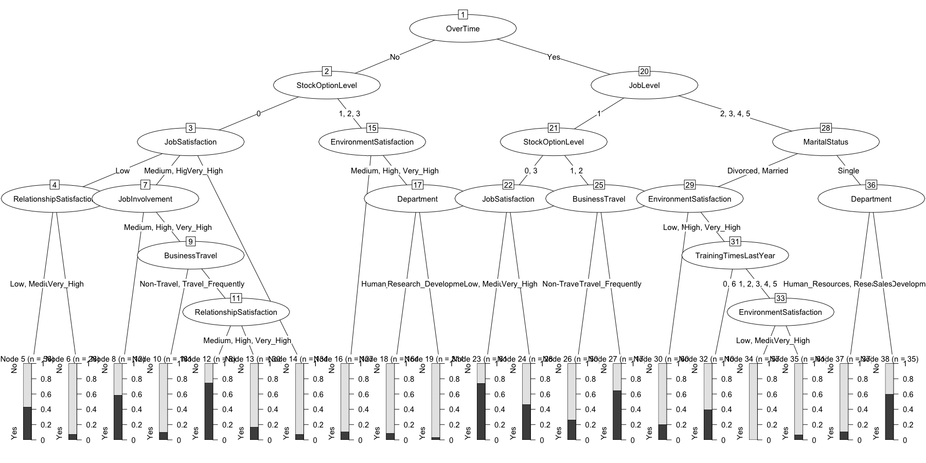
plot(chaidattrit1)
chisq.test(newattrit$Attrition, newattrit$OverTime)
##
##  Pearson's Chi-squared test with Yates' continuity correction
##
## data:  newattrit$Attrition and newattrit$OverTime
## X-squared = 87.564, df = 1, p-value < 2.2e-16
I happen to be a visual learner and prefer the plot to the print but
they are obviously reporting the same information so use them as you see
fit. As you can see the very first split it decides on is overtime yes
or no. I’ve run the chi-square test so that you can see the p value is
indeed very small (0.00000000000000022).
So the algorithm has decided that the most predictive way to divide our sample of employees is into 20 terminal nodes or buckets. Each one of the nodes represents a distinct set of predictors. Take a minute to look at node 19. Every person there shares the following characteristics.
- [2] OverTime in No
- [15] StockOptionLevel in 1, 2, 3
- [17] EnvironmentSatisfaction in Medium, High, Very_High
- [19] Department in Research_Development: No
There are n = 314 in this group, our prediction is that No they will
not attrit and we were “wrong” err = 3.2%. That’s some useful
information. To quote an old Star Wars movie “These are not the droids
you’re looking for…”. In other words, this is not a group we should be
overly worried about losing and we can say that with pretty high
confidence.
For contrast let’s look at node #23:
- [20] OverTime in Yes
- [21] JobLevel in 1
- [22] StockOptionLevel in 0, 3
- [23] JobSatisfaction in Low, Medium, High:
Where there are n = 61 staff, we predict they will leave Yes and we
get it wrong err = 26.2% of the time. A little worrisome that we’re not
as accurate but this is a group that bears watching or intervention if
we want to retain them.
Some other things to note. Because the predictors are considered
categorical we will get splits like we do for node 22, where 0 and 3 are
on one side and 1, 2 is on the other. The number of people in any node
can be quite variable. Finally, notice that a variable can occur at
different levels of the model like StockOptionLevel does!
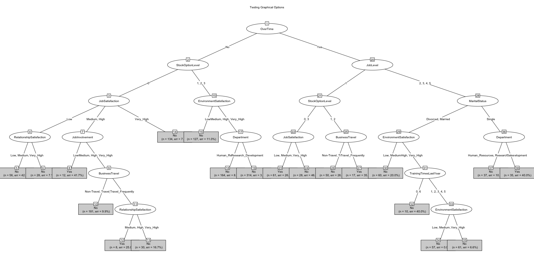
On the plot side of things there are a few key options you can adjust
to make things easier to read. The next blocks of code show you how to
adjust some key options such as adding a title, reducing the font size,
using “simple” mode, and changing colors.
# digress for plotting
plot(chaidattrit1, type = "simple")
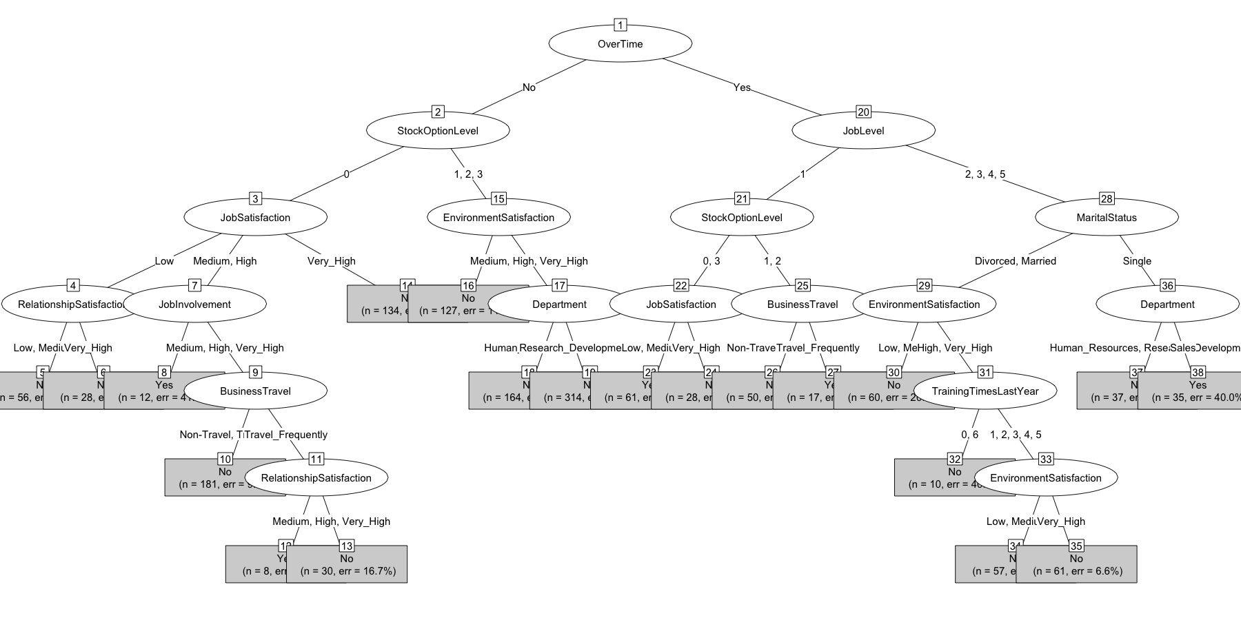
plot(
  chaidattrit1,
  main = "Testing Graphical Options",
  gp = gpar(fontsize = 8),
  type = "simple"
)
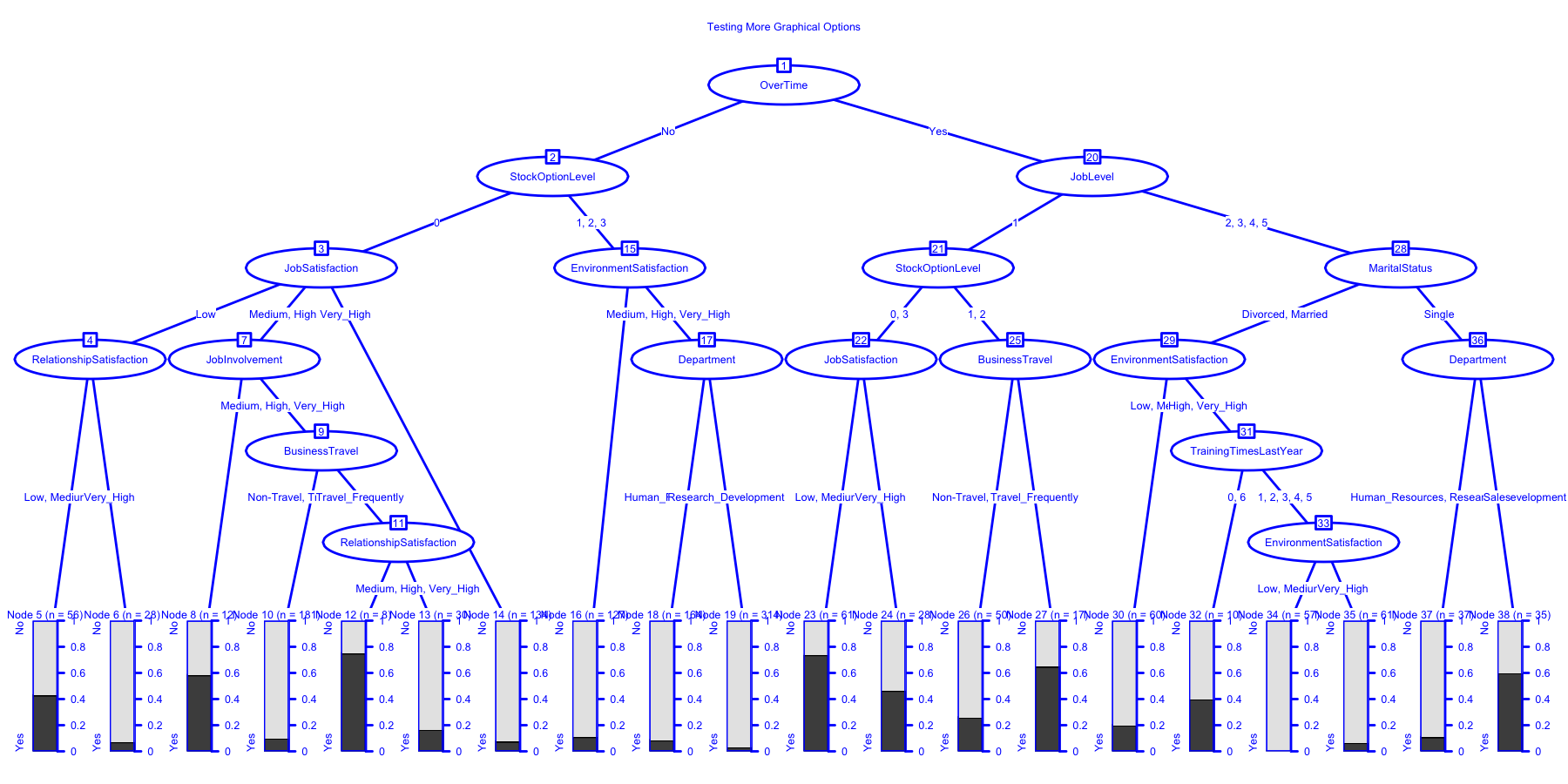
plot(
  chaidattrit1,
  main = "Testing More Graphical Options",
  gp = gpar(
    col = "blue",
    lty = "solid",
    lwd = 3,
    fontsize = 10
  )
)
Exercising some control
Next let’s look into varying the parameters chaid uses to build the
model. chaid_control (not surprisingly) controls the behavior of the
model building. When you check the documentation at ?chaid_control you
can see the list of 8 parameters you can adjust. We’ve already run the
default settings implicitly when we built chaidattrit1 let’s look at
three others.
minsplit- Number of observations in splitted response at which no further split is desired.minprob- Minimum frequency of observations in terminal nodes.maxheight- Maximum height for the tree.
We’ll use those but our fourth model we’ll simply require a higher significance level for alpha2 and alpha4.
ctrl <- chaid_control(minsplit = 200, minprob = 0.05)
ctrl # notice the rest of the list is there at the default value
## $alpha2
## [1] 0.05
##
## $alpha3
## [1] -1
##
## $alpha4
## [1] 0.05
##
## $minsplit
## [1] 200
##
## $minbucket
## [1] 7
##
## $minprob
## [1] 0.05
##
## $stump
## [1] FALSE
##
## $maxheight
## [1] -1
##
## attr(,"class")
## [1] "chaid_control"
chaidattrit2 <- chaid(Attrition ~ ., data = newattrit, control = ctrl)
print(chaidattrit2)
##
## Model formula:
## Attrition ~ BusinessTravel + Department + Education + EducationField +
##     EnvironmentSatisfaction + Gender + JobInvolvement + JobLevel +
##     JobRole + JobSatisfaction + MaritalStatus + NumCompaniesWorked +
##     OverTime + PerformanceRating + RelationshipSatisfaction +
##     StockOptionLevel + TrainingTimesLastYear + WorkLifeBalance
##
## Fitted party:
## [1] root
## |   [2] OverTime in No
## |   |   [3] StockOptionLevel in 0
## |   |   |   [4] JobSatisfaction in Low: No (n = 84, err = 31.0%)
## |   |   |   [5] JobSatisfaction in Medium, High
## |   |   |   |   [6] JobInvolvement in Low: Yes (n = 12, err = 41.7%)
## |   |   |   |   [7] JobInvolvement in Medium, High, Very_High
## |   |   |   |   |   [8] BusinessTravel in Non-Travel, Travel_Rarely: No (n = 181, err = 9.9%)
## |   |   |   |   |   [9] BusinessTravel in Travel_Frequently: No (n = 38, err = 28.9%)
## |   |   |   [10] JobSatisfaction in Very_High: No (n = 134, err = 7.5%)
## |   |   [11] StockOptionLevel in 1, 2, 3
## |   |   |   [12] EnvironmentSatisfaction in Low: No (n = 127, err = 11.0%)
## |   |   |   [13] EnvironmentSatisfaction in Medium, High, Very_High
## |   |   |   |   [14] Department in Human_Resources, Sales: No (n = 164, err = 8.5%)
## |   |   |   |   [15] Department in Research_Development: No (n = 314, err = 3.2%)
## |   [16] OverTime in Yes
## |   |   [17] JobLevel in 1: Yes (n = 156, err = 47.4%)
## |   |   [18] JobLevel in 2, 3, 4, 5
## |   |   |   [19] MaritalStatus in Divorced, Married: No (n = 188, err = 10.6%)
## |   |   |   [20] MaritalStatus in Single: No (n = 72, err = 34.7%)
##
## Number of inner nodes:     9
## Number of terminal nodes: 11
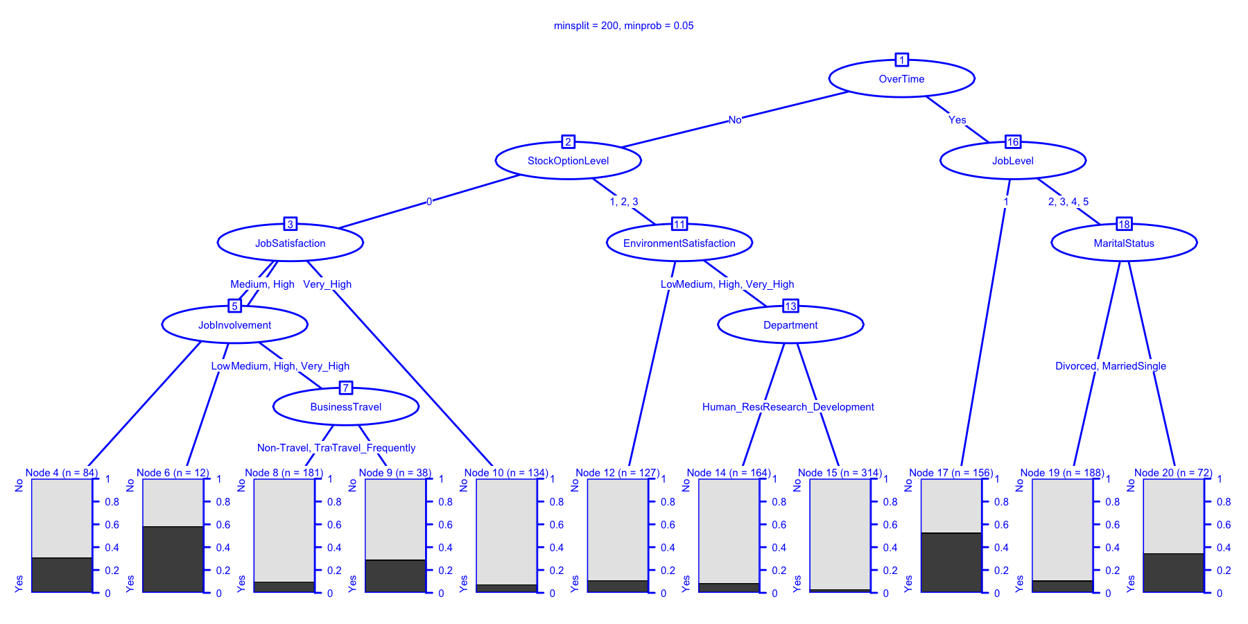
plot(
  chaidattrit2,
  main = "minsplit = 200, minprob = 0.05",
  gp = gpar(
    col = "blue",
    lty = "solid",
    lwd = 3  )
)
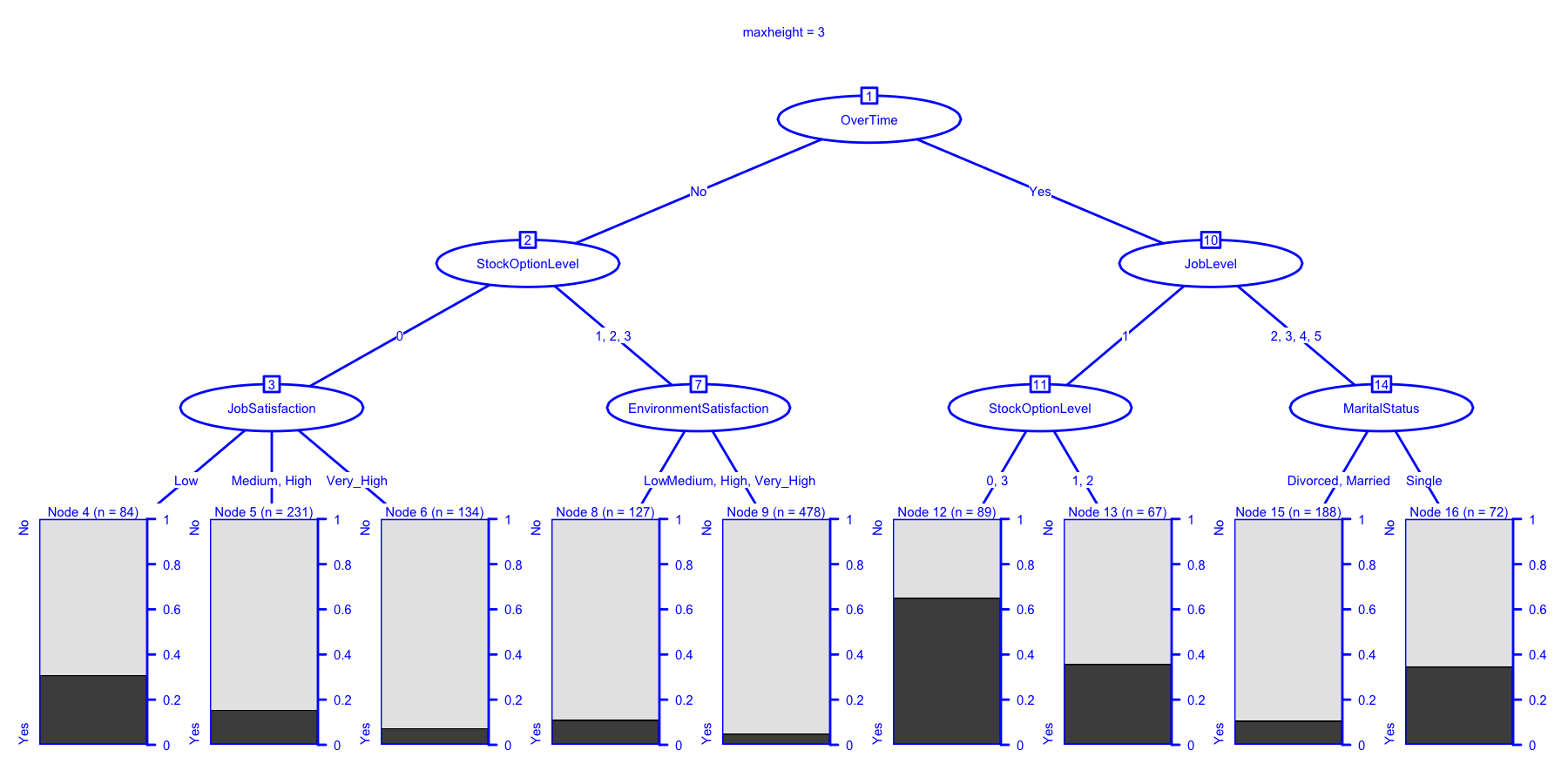
ctrl <- chaid_control(maxheight = 3)
chaidattrit3 <- chaid(Attrition ~ ., data = newattrit, control = ctrl)
print(chaidattrit3)
##
## Model formula:
## Attrition ~ BusinessTravel + Department + Education + EducationField +
##     EnvironmentSatisfaction + Gender + JobInvolvement + JobLevel +
##     JobRole + JobSatisfaction + MaritalStatus + NumCompaniesWorked +
##     OverTime + PerformanceRating + RelationshipSatisfaction +
##     StockOptionLevel + TrainingTimesLastYear + WorkLifeBalance
##
## Fitted party:
## [1] root
## |   [2] OverTime in No
## |   |   [3] StockOptionLevel in 0
## |   |   |   [4] JobSatisfaction in Low: No (n = 84, err = 31.0%)
## |   |   |   [5] JobSatisfaction in Medium, High: No (n = 231, err = 15.6%)
## |   |   |   [6] JobSatisfaction in Very_High: No (n = 134, err = 7.5%)
## |   |   [7] StockOptionLevel in 1, 2, 3
## |   |   |   [8] EnvironmentSatisfaction in Low: No (n = 127, err = 11.0%)
## |   |   |   [9] EnvironmentSatisfaction in Medium, High, Very_High: No (n = 478, err = 5.0%)
## |   [10] OverTime in Yes
## |   |   [11] JobLevel in 1
## |   |   |   [12] StockOptionLevel in 0, 3: Yes (n = 89, err = 34.8%)
## |   |   |   [13] StockOptionLevel in 1, 2: No (n = 67, err = 35.8%)
## |   |   [14] JobLevel in 2, 3, 4, 5
## |   |   |   [15] MaritalStatus in Divorced, Married: No (n = 188, err = 10.6%)
## |   |   |   [16] MaritalStatus in Single: No (n = 72, err = 34.7%)
##
## Number of inner nodes:    7
## Number of terminal nodes: 9
plot(
  chaidattrit3,
  main = "maxheight = 3",
  gp = gpar(
    col = "blue",
    lty = "solid",
    lwd = 3  )
)
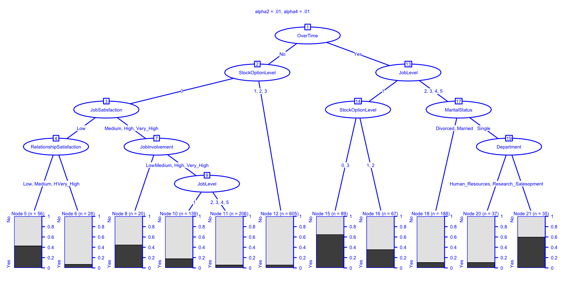
ctrl <- chaid_control(alpha2 = .01, alpha4 = .01)
chaidattrit4 <- chaid(Attrition ~ ., data = newattrit, control = ctrl)
print(chaidattrit4)
##
## Model formula:
## Attrition ~ BusinessTravel + Department + Education + EducationField +
##     EnvironmentSatisfaction + Gender + JobInvolvement + JobLevel +
##     JobRole + JobSatisfaction + MaritalStatus + NumCompaniesWorked +
##     OverTime + PerformanceRating + RelationshipSatisfaction +
##     StockOptionLevel + TrainingTimesLastYear + WorkLifeBalance
##
## Fitted party:
## [1] root
## |   [2] OverTime in No
## |   |   [3] StockOptionLevel in 0
## |   |   |   [4] JobSatisfaction in Low
## |   |   |   |   [5] RelationshipSatisfaction in Low, Medium, High: No (n = 56, err = 42.9%)
## |   |   |   |   [6] RelationshipSatisfaction in Very_High: No (n = 28, err = 7.1%)
## |   |   |   [7] JobSatisfaction in Medium, High, Very_High
## |   |   |   |   [8] JobInvolvement in Low: No (n = 20, err = 45.0%)
## |   |   |   |   [9] JobInvolvement in Medium, High, Very_High
## |   |   |   |   |   [10] JobLevel in 1: No (n = 139, err = 18.0%)
## |   |   |   |   |   [11] JobLevel in 2, 3, 4, 5: No (n = 206, err = 5.8%)
## |   |   [12] StockOptionLevel in 1, 2, 3: No (n = 605, err = 6.3%)
## |   [13] OverTime in Yes
## |   |   [14] JobLevel in 1
## |   |   |   [15] StockOptionLevel in 0, 3: Yes (n = 89, err = 34.8%)
## |   |   |   [16] StockOptionLevel in 1, 2: No (n = 67, err = 35.8%)
## |   |   [17] JobLevel in 2, 3, 4, 5
## |   |   |   [18] MaritalStatus in Divorced, Married: No (n = 188, err = 10.6%)
## |   |   |   [19] MaritalStatus in Single
## |   |   |   |   [20] Department in Human_Resources, Research_Development: No (n = 37, err = 10.8%)
## |   |   |   |   [21] Department in Sales: Yes (n = 35, err = 40.0%)
##
## Number of inner nodes:    10
## Number of terminal nodes: 11
plot(
  chaidattrit4,
  main = "alpha2 = .01, alpha4 = .01",
  gp = gpar(
    col = "blue",
    lty = "solid",
    lwd = 3  )
)
Let me call your attention to chaidattrit3 for a minute to highlight
two important things. First it is a good picture of what we get for
answer if we were to ask a question about what are the most important
predictors, what variables should we focus on. An important technical
detail has emerged as well. Notice that when you look at inner node #3
that there is no technical reason why a node has to have a binary
split in chaid. As this example clearly shows node#3 leads to a three
way split that is nodes #4-6.
How good is our model?
So the obvious question is which model is best? IMHO the joy of CHAID is in giving you a clear picture of what you would predict given the data and why. Then of course there is the usual problem every data scientist has, which is, I have what I think is a great model. How well will it generalize to new data? Whether that’s next years attrition numbers for the same company or say data from a different company.
But it’s time to talk about accuracy and all the related ideas, so on with the show…
When it’s all said and done we built a model called chaidattrit1 to be
able to predict or classify the 1,470 staff members. Seems reasonable
then that we can get back these predictions from the model for all 1,470
people and see how we did compared to the data we have about whether
they attrited or not. The print and plot commands sort of summarize that
for us at the terminal node level with an error rate but all in all
which of our four models is best?
The first step is to get the predictions for each model and put them
somewhere. For that we’ll use the predict command. If you inspect the
object you create (in my case with a head command) you’ll see it’s a
vector of factors where the attribute names is set to be the terminal
node the prediction is associated with. So pmodel1 <-
predict(chaidattrit1) puts our predictions using the first model we
built in a nice orderly fashion. On the other side newattrit$Attrition
has the actual outcome of whether the employee departed or not.
What we want is a comparison of how well we did. How often did we get it
right or wrong? Turns out what we need is called a confusion matrix. The
caret package has a function called confusionMatrix that will give
us what we want nicely formatted and printed.
There’s a nice short summary of what is produced at this url Confusion Matrix, so I won’t even try to repeat that material. I’ll just run the appropriate commands. Later we’ll revisit this topic to be more efficient. For now I want to focus on the results.
# digress how accurate were we
pmodel1 <-
predict(chaidattrit1)
head(pmodel1)
##  38  19  23  23  16  14
## Yes  No Yes Yes  No  No
## Levels: No Yes
pmodel2 <- predict(chaidattrit2)
pmodel3 <- predict(chaidattrit3)
pmodel4 <- predict(chaidattrit4)
confusionMatrix(pmodel1, newattrit$Attrition)
## Confusion Matrix and Statistics
##
##           Reference
## Prediction   No  Yes
##        No  1190  147
##        Yes   43   90
##
##                Accuracy : 0.8707
##                  95% CI : (0.8525, 0.8875)
##     No Information Rate : 0.8388
##     P-Value [Acc > NIR] : 0.0003553
##
##                   Kappa : 0.4192
##  Mcnemar's Test P-Value : 7.874e-14
##
##             Sensitivity : 0.9651
##             Specificity : 0.3797
##          Pos Pred Value : 0.8901
##          Neg Pred Value : 0.6767
##              Prevalence : 0.8388
##          Detection Rate : 0.8095
##    Detection Prevalence : 0.9095
##       Balanced Accuracy : 0.6724
##
##        'Positive' Class : No
##
confusionMatrix(pmodel2, newattrit$Attrition)
## Confusion Matrix and Statistics
##
##           Reference
## Prediction   No  Yes
##        No  1154  148
##        Yes   79   89
##
##                Accuracy : 0.8456
##                  95% CI : (0.8261, 0.8637)
##     No Information Rate : 0.8388
##     P-Value [Acc > NIR] : 0.2516
##
##                   Kappa : 0.353
##  Mcnemar's Test P-Value : 6.382e-06
##
##             Sensitivity : 0.9359
##             Specificity : 0.3755
##          Pos Pred Value : 0.8863
##          Neg Pred Value : 0.5298
##              Prevalence : 0.8388
##          Detection Rate : 0.7850
##    Detection Prevalence : 0.8857
##       Balanced Accuracy : 0.6557
##
##        'Positive' Class : No
##
confusionMatrix(pmodel3, newattrit$Attrition)
## Confusion Matrix and Statistics
##
##           Reference
## Prediction   No  Yes
##        No  1202  179
##        Yes   31   58
##
##                Accuracy : 0.8571
##                  95% CI : (0.8382, 0.8746)
##     No Information Rate : 0.8388
##     P-Value [Acc > NIR] : 0.02864
##
##                   Kappa : 0.2936
##  Mcnemar's Test P-Value : < 2e-16
##
##             Sensitivity : 0.9749
##             Specificity : 0.2447
##          Pos Pred Value : 0.8704
##          Neg Pred Value : 0.6517
##              Prevalence : 0.8388
##          Detection Rate : 0.8177
##    Detection Prevalence : 0.9395
##       Balanced Accuracy : 0.6098
##
##        'Positive' Class : No
##
confusionMatrix(pmodel4, newattrit$Attrition)
## Confusion Matrix and Statistics
##
##           Reference
## Prediction   No  Yes
##        No  1188  158
##        Yes   45   79
##
##                Accuracy : 0.8619
##                  95% CI : (0.8432, 0.8791)
##     No Information Rate : 0.8388
##     P-Value [Acc > NIR] : 0.007845
##
##                   Kappa : 0.3676
##  Mcnemar's Test P-Value : 3.815e-15
##
##             Sensitivity : 0.9635
##             Specificity : 0.3333
##          Pos Pred Value : 0.8826
##          Neg Pred Value : 0.6371
##              Prevalence : 0.8388
##          Detection Rate : 0.8082
##    Detection Prevalence : 0.9156
##       Balanced Accuracy : 0.6484
##
##        'Positive' Class : No
##
There we have it, four matrices, one for each of the models we made with
the different control parameters. It helpfully provides not just
Accuracy but also other common measures you may be interested in. I
won’t review them all that’s why I provided the link to a detailed
description
of all the measures. Before we leave the topic for a bit however, I do
want to highlight a way you can use the purrr package to make your
life a lot easier. A special thanks to Steven at
MungeX-3D for his recent post on purrr
which got me thinking about it.
We have 4 models so far (with more to come) we have the nice neat output
from caret but honestly to compare values across the 4 models involves
way too much scrolling back and forth right now. Let’s use purrr to
create a nice neat dataframe. purrr’s map command is like lapply
from base R, designed to apply some operations or functions to a list of
objects. So what we’ll do is as follows:
- Create a named list called
modellistto point to our four existing models (perhaps at a latter date we’ll start even earlier in our modelling process). - It’s a named list so we can name each model (for now with the accurate but uninteresting name Modelx)
- Pass the list using
mapto thepredictfunction to generate our predictions - Pipe
%>%those results to theconfusionMatrixfunction withmap - Pipe
%>%the confusion matrix results to map_dfr. The results of confusionMattrix are actually a list of six items. The ones we want to capture are in$overalland$byClass. We grab them, transpose them, and make them into a dataframe then bind the two dataframes together so everything is neatly packaged. The.id = ModelNumbtellsmap_dfrto add an identifying column to the dataframe. It is populated with the name of the list item we passed inmodellist. Therefore the object CHAIDresults contains everything we might want to use to compare models in one neat dataframe.
The kable call is simply for your reading convenience. Makes it a
little easier to read than a traditional print call.
library(kableExtra)
modellist <- list(Model1 = chaidattrit1, Model2 = chaidattrit2, Model3 = chaidattrit3, Model4 = chaidattrit4)
CHAIDResults <- map(modellist, ~ predict(.x)) %>%
                  map(~ confusionMatrix(newattrit$Attrition, .x)) %>%
                  map_dfr(~ cbind(as.data.frame(t(.x$overall)),as.data.frame(t(.x$byClass))), .id = "ModelNumb")
 kable(CHAIDResults, "html") %>%
   kable_styling(bootstrap_options = c("striped", "hover", "condensed", "responsive"),
                 font_size = 9)
| ModelNumb | Accuracy | Kappa | AccuracyLower | AccuracyUpper | AccuracyNull | AccuracyPValue | McnemarPValue | Sensitivity | Specificity | Pos Pred Value | Neg Pred Value | Precision | Recall | F1 | Prevalence | Detection Rate | Detection Prevalence | Balanced Accuracy |
|---|---|---|---|---|---|---|---|---|---|---|---|---|---|---|---|---|---|---|
| Model1 | 0.8707483 | 0.4191632 | 0.8525159 | 0.8874842 | 0.9095238 | 0.9999996 | 0.0e+00 | 0.8900524 | 0.6766917 | 0.9651257 | 0.3797468 | 0.9651257 | 0.8900524 | 0.9260700 | 0.9095238 | 0.8095238 | 0.8387755 | 0.7833720 |
| Model2 | 0.8455782 | 0.3529603 | 0.8260781 | 0.8636860 | 0.8857143 | 0.9999985 | 6.4e-06 | 0.8863287 | 0.5297619 | 0.9359286 | 0.3755274 | 0.9359286 | 0.8863287 | 0.9104536 | 0.8857143 | 0.7850340 | 0.8387755 | 0.7080453 |
| Model3 | 0.8571429 | 0.2936476 | 0.8382017 | 0.8746440 | 0.9394558 | 1.0000000 | 0.0e+00 | 0.8703838 | 0.6516854 | 0.9748581 | 0.2447257 | 0.9748581 | 0.8703838 | 0.9196634 | 0.9394558 | 0.8176871 | 0.8387755 | 0.7610346 |
| Model4 | 0.8619048 | 0.3676334 | 0.8432050 | 0.8791447 | 0.9156463 | 1.0000000 | 0.0e+00 | 0.8826152 | 0.6370968 | 0.9635036 | 0.3333333 | 0.9635036 | 0.8826152 | 0.9212873 | 0.9156463 | 0.8081633 | 0.8387755 | 0.7598560 |
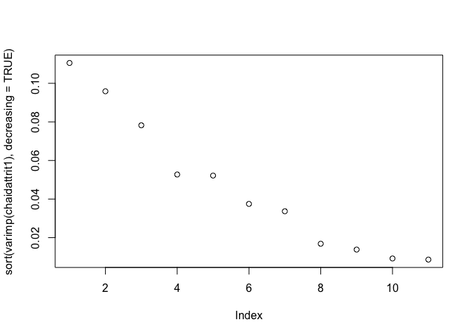
One other thing I’ll mention in passing is that the partykit package
offers a way of assessing the relative importance of the variables in
the model via the varimp command. We’ll come back to this concept of
variable importance later but for now a simple example of text and plot
output.
sort(varimp(chaidattrit1), decreasing = TRUE)
##                 JobLevel                 OverTime  EnvironmentSatisfaction
##              0.142756888              0.114384725              0.071069051
##         StockOptionLevel            MaritalStatus          JobSatisfaction
##              0.058726463              0.030332565              0.029157845
##    TrainingTimesLastYear RelationshipSatisfaction               Department
##              0.025637743              0.015700750              0.013815233
##           BusinessTravel           JobInvolvement
##              0.009906245              0.009205317
plot(sort(varimp(chaidattrit1), decreasing = TRUE))
What about those other variables?
But before we go much farther we should probably circle back and make
use of all those variables that were coded as integers that we
conveniently ignored in building our first four models. Let’s bring them
into our model building activities and see what they can add to our
understanding. As a first step let’s use ggplot2 and take a look at
their distribution using a density plot.
# Turning numeric variables into factors
## what do they look like
attrition %>%
  select_if(is.numeric) %>%
  gather(metric, value) %>%
  ggplot(aes(value, fill = metric)) +
  geom_density(show.legend = FALSE) +
  facet_wrap( ~ metric, scales = "free")
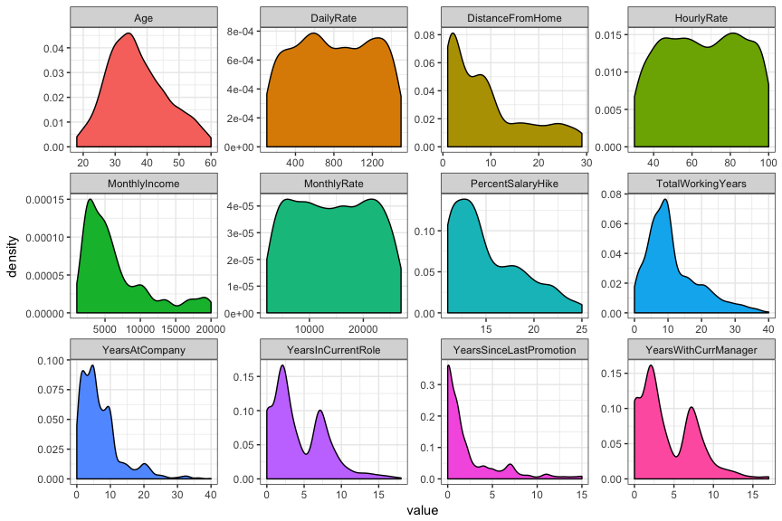
Well other than Age very few of those variables appear to have
especially normal distributions. That’s okay we’re going to wind up
cutting them up into factors anyway. The only question is what are the
best cut-points to use? In base R the cut function default is equal
intervals (distances along the x axis). You can also specify your own
cutpoints and your own labels as shown below.
table(cut(attrition$YearsWithCurrManager, breaks = 5))
##
## (-0.017,3.4]    (3.4,6.8]   (6.8,10.2]  (10.2,13.6]    (13.6,17]
##          825          158          414           54           19
table(attrition$YearsSinceLastPromotion)
##
##   0   1   2   3   4   5   6   7   8   9  10  11  12  13  14  15
## 581 357 159  52  61  45  32  76  18  17   6  24  10  10   9  13
table(cut(
  attrition$YearsSinceLastPromotion,
  breaks = c(-1, 0.9, 1.9, 2.9, 30),
  labels = c("Less than 1", "1", "2", "More than 2")
))
##
## Less than 1           1           2 More than 2
##         581         357         159         373
ggplot2 has three helper functions I prefer to use: cut_interval,
cut_number, and cut_width. cut_interval makes n groups with equal
range, cut_number makes n groups with (approximately) equal numbers of
observations, and cut_width makes groups of a fixed specified width.
As we think about moving the numeric variables into factors any of these
might be a viable alternative.
# cut_interval makes n groups with equal range
table(cut_interval(attrition$YearsWithCurrManager, n = 5))
##
##     [0,3.4]   (3.4,6.8]  (6.8,10.2] (10.2,13.6]   (13.6,17]
##         825         158         414          54          19
# cut_number makes n groups with (approximately) equal numbers of observations
table(cut_number(attrition$YearsWithCurrManager, n = 5))
##
##  [0,1]  (1,2]  (2,4]  (4,7] (7,17]
##    339    344    240    276    271
# cut_width makes groups of width width
table(cut_width(attrition$YearsWithCurrManager, width = 2))
##
##  [-1,1]   (1,3]   (3,5]   (5,7]   (7,9]  (9,11] (11,13] (13,15] (15,17]
##     339     486     129     245     171      49      32      10       9
For the sake of our current example let’s say that I would like to focus
on groups of more or less equal size which means that I would need to
apply cut_number to each of the 12 variables under discussion. I’m not
enamored of running the function 12 times though so I would prefer to
wrap it in a mutate_if statement. If the variable is numeric then
apply cut_number with n=5.
The problem is that cut_number will error out if it doesn’t think
there are enough values to produce the bins you requested. So…
cut_number(attrition$YearsWithCurrManager, n = 6)
# Error: Insufficient data values to produce 6 bins.
cut_number(attrition$YearsSinceLastPromotion, n = 4)
# Error: Insufficient data values to produce 4 bins.
attrition %>%
  mutate_if(is.numeric, funs(cut_number(., n=5)))
# Error in mutate_impl(.data, dots) :
#   Evaluation error: Insufficient data values to produce 5 bins..
A little sleuthing reveals that there is one variable among the 12 that
has too few values for the cut_number function to work. That variable
is YearsSinceLastPromotion. Let’s try what we would like but
explicitly select out that variable.
attrition %>%
  select(-YearsSinceLastPromotion) %>%
  mutate_if(is.numeric, funs(cut_number(., n=5))) %>% head
##       Age Attrition    BusinessTravel          DailyRate
## 1 (38,45]       Yes     Travel_Rarely     (942,1.22e+03]
## 2 (45,60]        No Travel_Frequently          [102,392]
## 3 (34,38]       Yes     Travel_Rarely (1.22e+03,1.5e+03]
## 4 (29,34]        No Travel_Frequently (1.22e+03,1.5e+03]
## 5 [18,29]        No     Travel_Rarely          (392,656]
## 6 (29,34]        No Travel_Frequently     (942,1.22e+03]
##             Department DistanceFromHome     Education EducationField
## 1                Sales            [1,2]       College  Life_Sciences
## 2 Research_Development            (5,9] Below_College  Life_Sciences
## 3 Research_Development            [1,2]       College          Other
## 4 Research_Development            (2,5]        Master  Life_Sciences
## 5 Research_Development            [1,2] Below_College        Medical
## 6 Research_Development            [1,2]       College  Life_Sciences
##   EnvironmentSatisfaction Gender HourlyRate JobInvolvement JobLevel
## 1                  Medium Female   (87,100]           High        2
## 2                    High   Male    (59,73]         Medium        2
## 3               Very_High   Male   (87,100]         Medium        1
## 4               Very_High Female    (45,59]           High        1
## 5                     Low   Male    [30,45]           High        1
## 6               Very_High   Male    (73,87]           High        1
##                 JobRole JobSatisfaction MaritalStatus       MonthlyIncome
## 1       Sales_Executive       Very_High        Single (5.74e+03,9.86e+03]
## 2    Research_Scientist          Medium       Married (4.23e+03,5.74e+03]
## 3 Laboratory_Technician            High        Single  [1.01e+03,2.7e+03]
## 4    Research_Scientist            High       Married  (2.7e+03,4.23e+03]
## 5 Laboratory_Technician          Medium       Married  (2.7e+03,4.23e+03]
## 6 Laboratory_Technician       Very_High        Single  (2.7e+03,4.23e+03]
##           MonthlyRate NumCompaniesWorked OverTime PercentSalaryHike
## 1 (1.67e+04,2.17e+04]                  8      Yes           [11,12]
## 2  (2.17e+04,2.7e+04]                  1       No           (19,25]
## 3 [2.09e+03,6.89e+03]                  6      Yes           (13,15]
## 4  (2.17e+04,2.7e+04]                  1      Yes           [11,12]
## 5 (1.18e+04,1.67e+04]                  9       No           [11,12]
## 6 (1.18e+04,1.67e+04]                  0       No           (12,13]
##   PerformanceRating RelationshipSatisfaction StockOptionLevel
## 1         Excellent                      Low                0
## 2       Outstanding                Very_High                1
## 3         Excellent                   Medium                0
## 4         Excellent                     High                0
## 5         Excellent                Very_High                1
## 6         Excellent                     High                0
##   TotalWorkingYears TrainingTimesLastYear WorkLifeBalance YearsAtCompany
## 1             (5,8]                     0             Bad          (5,7]
## 2            (8,10]                     3          Better         (7,10]
## 3             (5,8]                     3          Better          [0,2]
## 4             (5,8]                     3          Better         (7,10]
## 5             (5,8]                     3          Better          [0,2]
## 6             (5,8]                     2            Good          (5,7]
##   YearsInCurrentRole YearsWithCurrManager
## 1              (2,4]                (4,7]
## 2              (4,7]                (4,7]
## 3              [0,1]                [0,1]
## 4              (4,7]                [0,1]
## 5              (1,2]                (1,2]
## 6              (4,7]                (4,7]
Yes that appears to be it. So let’s manually cut it into 4 groups and
then apply the 5 grouping code to the other 11 variables. Once we have
accomplished that we can run the same newattrit <- attrition %>%
select_if(is.factor) we ran earlier to produce a newattrit dataframe
we can work with.
attrition$YearsSinceLastPromotion <- cut(
attrition$YearsSinceLastPromotion,
breaks = c(-1, 0.9, 1.9, 2.9, 30),
labels = c("Less than 1", "1", "2", "More than 2")
)
attrition <- attrition %>%
mutate_if(is.numeric, funs(cut_number(., n=5)))
summary(attrition)
## Age Attrition BusinessTravel
## [18,29]:326 No :1233 Non-Travel : 150
## (29,34]:325 Yes: 237 Travel_Frequently: 277
## (34,38]:255 Travel_Rarely :1043
## (38,45]:291
## (45,60]:273
##
##
## DailyRate Department DistanceFromHome
## [102,392] :294 Human_Resources : 63 [1,2] :419
## (392,656] :294 Research_Development:961 (2,5] :213
## (656,942] :294 Sales :446 (5,9] :308
## (942,1.22e+03] :294 (9,17] :253
## (1.22e+03,1.5e+03]:294 (17,29]:277
##
##
## Education EducationField EnvironmentSatisfaction
## Below_College:170 Human_Resources : 27 Low :284
## College :282 Life_Sciences :606 Medium :287
## Bachelor :572 Marketing :159 High :453
## Master :398 Medical :464 Very_High:446
## Doctor : 48 Other : 82
## Technical_Degree:132
##
## Gender HourlyRate JobInvolvement JobLevel
## Female:588 [30,45] :306 Low : 83 1:543
## Male :882 (45,59] :298 Medium :375 2:534
## (59,73] :280 High :868 3:218
## (73,87] :312 Very_High:144 4:106
## (87,100]:274 5: 69
##
##
## JobRole JobSatisfaction MaritalStatus
## Sales_Executive :326 Low :289 Divorced:327
## Research_Scientist :292 Medium :280 Married :673
## Laboratory_Technician :259 High :442 Single :470
## Manufacturing_Director :145 Very_High:459
## Healthcare_Representative:131
## Manager :102
## (Other) :215
## MonthlyIncome MonthlyRate NumCompaniesWorked
## [1.01e+03,2.7e+03] :294 [2.09e+03,6.89e+03]:294 1 :521
## (2.7e+03,4.23e+03] :294 (6.89e+03,1.18e+04]:294 0 :197
## (4.23e+03,5.74e+03]:294 (1.18e+04,1.67e+04]:294 3 :159
## (5.74e+03,9.86e+03]:294 (1.67e+04,2.17e+04]:294 2 :146
## (9.86e+03,2e+04] :294 (2.17e+04,2.7e+04] :294 4 :139
## 7 : 74
## (Other):234
## OverTime PercentSalaryHike PerformanceRating RelationshipSatisfaction
## No :1054 [11,12]:408 Low : 0 Low :276
## Yes: 416 (12,13]:209 Good : 0 Medium :303
## (13,15]:302 Excellent :1244 High :459
## (15,19]:325 Outstanding: 226 Very_High:432
## (19,25]:226
##
##
## StockOptionLevel TotalWorkingYears TrainingTimesLastYear WorkLifeBalance
## 0:631 [0,5] :316 0: 54 Bad : 80
## 1:596 (5,8] :309 1: 71 Good :344
## 2:158 (8,10] :298 2:547 Better:893
## 3: 85 (10,17]:261 3:491 Best :153
## (17,40]:286 4:123
## 5:119
## 6: 65
## YearsAtCompany YearsInCurrentRole YearsSinceLastPromotion
## [0,2] :342 [0,1] :301 Less than 1:581
## (2,5] :434 (1,2] :372 1 :357
## (5,7] :166 (2,4] :239 2 :159
## (7,10] :282 (4,7] :295 More than 2:373
## (10,40]:246 (7,18]:263
##
##
## YearsWithCurrManager
## [0,1] :339
## (1,2] :344
## (2,4] :240
## (4,7] :276
## (7,17]:271
##
##
newattrit <- attrition %>%
select_if(is.factor)
dim(newattrit)
## [1] 1470 31
Now we have newattrit with all 30 predictor variables. We will simply
repeat the process we used earlier to develop 4 new models.
# Repeat to produce models 5-8
chaidattrit5 <- chaid(Attrition ~ ., data = newattrit)
print(chaidattrit5)
##
## Model formula:
## Attrition ~ Age + BusinessTravel + DailyRate + Department + DistanceFromHome +
##     Education + EducationField + EnvironmentSatisfaction + Gender +
##     HourlyRate + JobInvolvement + JobLevel + JobRole + JobSatisfaction +
##     MaritalStatus + MonthlyIncome + MonthlyRate + NumCompaniesWorked +
##     OverTime + PercentSalaryHike + PerformanceRating + RelationshipSatisfaction +
##     StockOptionLevel + TotalWorkingYears + TrainingTimesLastYear +
##     WorkLifeBalance + YearsAtCompany + YearsInCurrentRole + YearsSinceLastPromotion +
##     YearsWithCurrManager
##
## Fitted party:
## [1] root
## |   [2] OverTime in No
## |   |   [3] YearsAtCompany in [0,2]
## |   |   |   [4] Age in [18,29], (29,34]
## |   |   |   |   [5] StockOptionLevel in 0
## |   |   |   |   |   [6] BusinessTravel in Non-Travel, Travel_Rarely: No (n = 56, err = 41.1%)
## |   |   |   |   |   [7] BusinessTravel in Travel_Frequently: Yes (n = 10, err = 10.0%)
## |   |   |   |   [8] StockOptionLevel in 1, 2, 3: No (n = 63, err = 15.9%)
## |   |   |   [9] Age in (34,38], (38,45], (45,60]
## |   |   |   |   [10] WorkLifeBalance in Bad: No (n = 4, err = 50.0%)
## |   |   |   |   [11] WorkLifeBalance in Good, Better, Best
## |   |   |   |   |   [12] EducationField in Human_Resources, Life_Sciences, Marketing, Medical: No (n = 92, err = 2.2%)
## |   |   |   |   |   [13] EducationField in Other, Technical_Degree: No (n = 13, err = 23.1%)
## |   |   [14] YearsAtCompany in (2,5], (5,7], (7,10], (10,40]
## |   |   |   [15] WorkLifeBalance in Bad: No (n = 45, err = 22.2%)
## |   |   |   [16] WorkLifeBalance in Good, Better, Best
## |   |   |   |   [17] JobSatisfaction in Low
## |   |   |   |   |   [18] StockOptionLevel in 0
## |   |   |   |   |   |   [19] RelationshipSatisfaction in Low: Yes (n = 11, err = 45.5%)
## |   |   |   |   |   |   [20] RelationshipSatisfaction in Medium: No (n = 12, err = 8.3%)
## |   |   |   |   |   |   [21] RelationshipSatisfaction in High: No (n = 17, err = 47.1%)
## |   |   |   |   |   |   [22] RelationshipSatisfaction in Very_High: No (n = 20, err = 0.0%)
## |   |   |   |   |   [23] StockOptionLevel in 1, 2, 3: No (n = 93, err = 4.3%)
## |   |   |   |   [24] JobSatisfaction in Medium, High, Very_High
## |   |   |   |   |   [25] Age in [18,29], (29,34], (34,38], (38,45]
## |   |   |   |   |   |   [26] BusinessTravel in Non-Travel, Travel_Rarely
## |   |   |   |   |   |   |   [27] JobInvolvement in Low: No (n = 25, err = 12.0%)
## |   |   |   |   |   |   |   [28] JobInvolvement in Medium, High, Very_High
## |   |   |   |   |   |   |   |   [29] RelationshipSatisfaction in Low: No (n = 81, err = 3.7%)
## |   |   |   |   |   |   |   |   [30] RelationshipSatisfaction in Medium, High: No (n = 198, err = 0.0%)
## |   |   |   |   |   |   |   |   [31] RelationshipSatisfaction in Very_High
## |   |   |   |   |   |   |   |   |   [32] DistanceFromHome in [1,2], (2,5], (5,9], (17,29]: No (n = 92, err = 2.2%)
## |   |   |   |   |   |   |   |   |   [33] DistanceFromHome in (9,17]: No (n = 13, err = 23.1%)
## |   |   |   |   |   |   [34] BusinessTravel in Travel_Frequently: No (n = 95, err = 8.4%)
## |   |   |   |   |   [35] Age in (45,60]
## |   |   |   |   |   |   [36] JobSatisfaction in Low, Medium, High
## |   |   |   |   |   |   |   [37] TotalWorkingYears in [0,5], (5,8], (8,10], (17,40]: No (n = 57, err = 0.0%)
## |   |   |   |   |   |   |   [38] TotalWorkingYears in (10,17]: No (n = 14, err = 28.6%)
## |   |   |   |   |   |   [39] JobSatisfaction in Very_High: No (n = 43, err = 20.9%)
## |   [40] OverTime in Yes
## |   |   [41] JobLevel in 1
## |   |   |   [42] StockOptionLevel in 0, 3
## |   |   |   |   [43] DistanceFromHome in [1,2], (2,5]
## |   |   |   |   |   [44] EnvironmentSatisfaction in Low: Yes (n = 12, err = 16.7%)
## |   |   |   |   |   [45] EnvironmentSatisfaction in Medium, High, Very_High: No (n = 33, err = 36.4%)
## |   |   |   |   [46] DistanceFromHome in (5,9], (9,17], (17,29]: Yes (n = 44, err = 18.2%)
## |   |   |   [47] StockOptionLevel in 1, 2
## |   |   |   |   [48] BusinessTravel in Non-Travel, Travel_Rarely: No (n = 50, err = 26.0%)
## |   |   |   |   [49] BusinessTravel in Travel_Frequently: Yes (n = 17, err = 35.3%)
## |   |   [50] JobLevel in 2, 3, 4, 5
## |   |   |   [51] MaritalStatus in Divorced, Married
## |   |   |   |   [52] EnvironmentSatisfaction in Low, Medium: No (n = 60, err = 20.0%)
## |   |   |   |   [53] EnvironmentSatisfaction in High, Very_High
## |   |   |   |   |   [54] TrainingTimesLastYear in 0, 6: No (n = 10, err = 40.0%)
## |   |   |   |   |   [55] TrainingTimesLastYear in 1, 2, 3, 4, 5
## |   |   |   |   |   |   [56] YearsInCurrentRole in [0,1], (1,2]: No (n = 36, err = 11.1%)
## |   |   |   |   |   |   [57] YearsInCurrentRole in (2,4], (4,7], (7,18]: No (n = 82, err = 0.0%)
## |   |   |   [58] MaritalStatus in Single
## |   |   |   |   [59] Department in Human_Resources, Research_Development: No (n = 37, err = 10.8%)
## |   |   |   |   [60] Department in Sales: Yes (n = 35, err = 40.0%)
##
## Number of inner nodes:    28
## Number of terminal nodes: 32
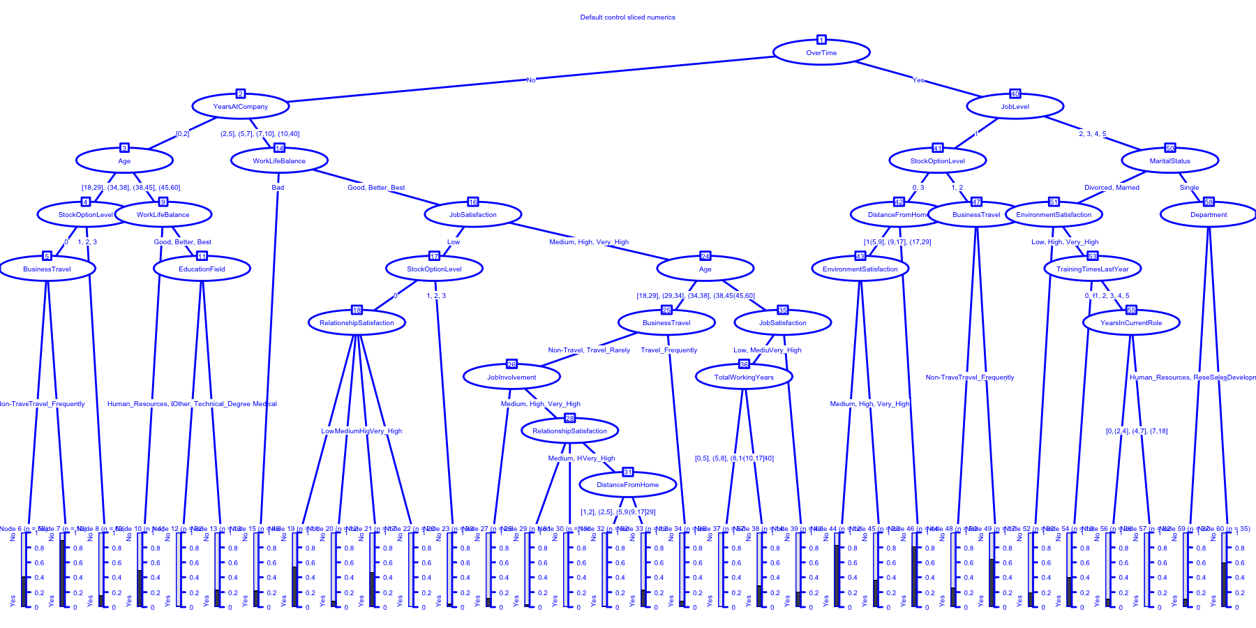
plot(
  chaidattrit5,
  main = "Default control sliced numerics",
  gp = gpar(
    col = "blue",
    lty = "solid",
    lwd = 3,
    fontsize = 8
  )
)
ctrl <- chaid_control(minsplit = 200, minprob = 0.05)
chaidattrit6 <- chaid(Attrition ~ ., data = newattrit, control = ctrl)
print(chaidattrit6)
##
## Model formula:
## Attrition ~ Age + BusinessTravel + DailyRate + Department + DistanceFromHome +
##     Education + EducationField + EnvironmentSatisfaction + Gender +
##     HourlyRate + JobInvolvement + JobLevel + JobRole + JobSatisfaction +
##     MaritalStatus + MonthlyIncome + MonthlyRate + NumCompaniesWorked +
##     OverTime + PercentSalaryHike + PerformanceRating + RelationshipSatisfaction +
##     StockOptionLevel + TotalWorkingYears + TrainingTimesLastYear +
##     WorkLifeBalance + YearsAtCompany + YearsInCurrentRole + YearsSinceLastPromotion +
##     YearsWithCurrManager
##
## Fitted party:
## [1] root
## |   [2] OverTime in No
## |   |   [3] YearsAtCompany in [0,2]
## |   |   |   [4] Age in [18,29], (29,34]: No (n = 129, err = 32.6%)
## |   |   |   [5] Age in (34,38], (38,45], (45,60]: No (n = 109, err = 6.4%)
## |   |   [6] YearsAtCompany in (2,5], (5,7], (7,10], (10,40]
## |   |   |   [7] WorkLifeBalance in Bad: No (n = 45, err = 22.2%)
## |   |   |   [8] WorkLifeBalance in Good, Better, Best
## |   |   |   |   [9] JobSatisfaction in Low: No (n = 153, err = 12.4%)
## |   |   |   |   [10] JobSatisfaction in Medium, High, Very_High
## |   |   |   |   |   [11] Age in [18,29], (29,34], (34,38], (38,45]
## |   |   |   |   |   |   [12] BusinessTravel in Non-Travel, Travel_Rarely
## |   |   |   |   |   |   |   [13] JobInvolvement in Low: No (n = 25, err = 12.0%)
## |   |   |   |   |   |   |   [14] JobInvolvement in Medium, High, Very_High
## |   |   |   |   |   |   |   |   [15] RelationshipSatisfaction in Low: No (n = 81, err = 3.7%)
## |   |   |   |   |   |   |   |   [16] RelationshipSatisfaction in Medium, High: No (n = 198, err = 0.0%)
## |   |   |   |   |   |   |   |   [17] RelationshipSatisfaction in Very_High: No (n = 105, err = 4.8%)
## |   |   |   |   |   |   [18] BusinessTravel in Travel_Frequently: No (n = 95, err = 8.4%)
## |   |   |   |   |   [19] Age in (45,60]: No (n = 114, err = 11.4%)
## |   [20] OverTime in Yes
## |   |   [21] JobLevel in 1: Yes (n = 156, err = 47.4%)
## |   |   [22] JobLevel in 2, 3, 4, 5
## |   |   |   [23] MaritalStatus in Divorced, Married: No (n = 188, err = 10.6%)
## |   |   |   [24] MaritalStatus in Single: No (n = 72, err = 34.7%)
##
## Number of inner nodes:    11
## Number of terminal nodes: 13
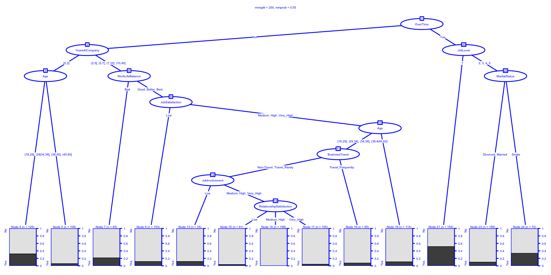
plot(
  chaidattrit6,
  main = "minsplit = 200, minprob = 0.05",
  gp = gpar(
    col = "blue",
    lty = "solid",
    lwd = 3,
    fontsize = 8
  )
)
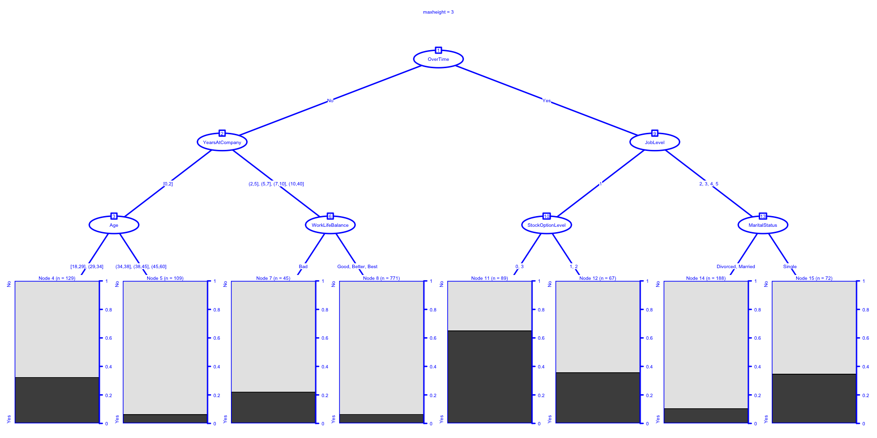
ctrl <- chaid_control(maxheight = 3)
chaidattrit7 <- chaid(Attrition ~ ., data = newattrit, control = ctrl)
print(chaidattrit7)
##
## Model formula:
## Attrition ~ Age + BusinessTravel + DailyRate + Department + DistanceFromHome +
##     Education + EducationField + EnvironmentSatisfaction + Gender +
##     HourlyRate + JobInvolvement + JobLevel + JobRole + JobSatisfaction +
##     MaritalStatus + MonthlyIncome + MonthlyRate + NumCompaniesWorked +
##     OverTime + PercentSalaryHike + PerformanceRating + RelationshipSatisfaction +
##     StockOptionLevel + TotalWorkingYears + TrainingTimesLastYear +
##     WorkLifeBalance + YearsAtCompany + YearsInCurrentRole + YearsSinceLastPromotion +
##     YearsWithCurrManager
##
## Fitted party:
## [1] root
## |   [2] OverTime in No
## |   |   [3] YearsAtCompany in [0,2]
## |   |   |   [4] Age in [18,29], (29,34]: No (n = 129, err = 32.6%)
## |   |   |   [5] Age in (34,38], (38,45], (45,60]: No (n = 109, err = 6.4%)
## |   |   [6] YearsAtCompany in (2,5], (5,7], (7,10], (10,40]
## |   |   |   [7] WorkLifeBalance in Bad: No (n = 45, err = 22.2%)
## |   |   |   [8] WorkLifeBalance in Good, Better, Best: No (n = 771, err = 6.6%)
## |   [9] OverTime in Yes
## |   |   [10] JobLevel in 1
## |   |   |   [11] StockOptionLevel in 0, 3: Yes (n = 89, err = 34.8%)
## |   |   |   [12] StockOptionLevel in 1, 2: No (n = 67, err = 35.8%)
## |   |   [13] JobLevel in 2, 3, 4, 5
## |   |   |   [14] MaritalStatus in Divorced, Married: No (n = 188, err = 10.6%)
## |   |   |   [15] MaritalStatus in Single: No (n = 72, err = 34.7%)
##
## Number of inner nodes:    7
## Number of terminal nodes: 8
plot(
  chaidattrit7,
  main = "maxheight = 3",
  gp = gpar(
    col = "blue",
    lty = "solid",
    lwd = 3,
    fontsize = 8
  )
)
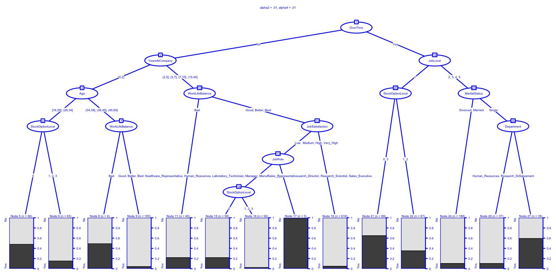
ctrl <- chaid_control(alpha2 = .01, alpha4 = .01)
chaidattrit8 <- chaid(Attrition ~ ., data = newattrit, control = ctrl)
print(chaidattrit8)
##
## Model formula:
## Attrition ~ Age + BusinessTravel + DailyRate + Department + DistanceFromHome +
##     Education + EducationField + EnvironmentSatisfaction + Gender +
##     HourlyRate + JobInvolvement + JobLevel + JobRole + JobSatisfaction +
##     MaritalStatus + MonthlyIncome + MonthlyRate + NumCompaniesWorked +
##     OverTime + PercentSalaryHike + PerformanceRating + RelationshipSatisfaction +
##     StockOptionLevel + TotalWorkingYears + TrainingTimesLastYear +
##     WorkLifeBalance + YearsAtCompany + YearsInCurrentRole + YearsSinceLastPromotion +
##     YearsWithCurrManager
##
## Fitted party:
## [1] root
## |   [2] OverTime in No
## |   |   [3] YearsAtCompany in [0,2]
## |   |   |   [4] Age in [18,29], (29,34]
## |   |   |   |   [5] StockOptionLevel in 0: No (n = 66, err = 48.5%)
## |   |   |   |   [6] StockOptionLevel in 1, 2, 3: No (n = 63, err = 15.9%)
## |   |   |   [7] Age in (34,38], (38,45], (45,60]
## |   |   |   |   [8] WorkLifeBalance in Bad: No (n = 4, err = 50.0%)
## |   |   |   |   [9] WorkLifeBalance in Good, Better, Best: No (n = 105, err = 4.8%)
## |   |   [10] YearsAtCompany in (2,5], (5,7], (7,10], (10,40]
## |   |   |   [11] WorkLifeBalance in Bad: No (n = 45, err = 22.2%)
## |   |   |   [12] WorkLifeBalance in Good, Better, Best
## |   |   |   |   [13] JobSatisfaction in Low
## |   |   |   |   |   [14] JobRole in Healthcare_Representative, Human_Resources, Laboratory_Technician, Manager, Manufacturing_Director, Research_Director, Research_Scientist, Sales_Executive
## |   |   |   |   |   |   [15] StockOptionLevel in 0: No (n = 58, err = 22.4%)
## |   |   |   |   |   |   [16] StockOptionLevel in 1, 2, 3: No (n = 92, err = 3.3%)
## |   |   |   |   |   [17] JobRole in Sales_Representative: Yes (n = 3, err = 0.0%)
## |   |   |   |   [18] JobSatisfaction in Medium, High, Very_High: No (n = 618, err = 5.2%)
## |   [19] OverTime in Yes
## |   |   [20] JobLevel in 1
## |   |   |   [21] StockOptionLevel in 0, 3: Yes (n = 89, err = 34.8%)
## |   |   |   [22] StockOptionLevel in 1, 2: No (n = 67, err = 35.8%)
## |   |   [23] JobLevel in 2, 3, 4, 5
## |   |   |   [24] MaritalStatus in Divorced, Married: No (n = 188, err = 10.6%)
## |   |   |   [25] MaritalStatus in Single
## |   |   |   |   [26] Department in Human_Resources, Research_Development: No (n = 37, err = 10.8%)
## |   |   |   |   [27] Department in Sales: Yes (n = 35, err = 40.0%)
##
## Number of inner nodes:    13
## Number of terminal nodes: 14
plot(
  chaidattrit8,
  main = "alpha2 = .01, alpha4 = .01",
  gp = gpar(
    col = "blue",
    lty = "solid",
    lwd = 3,
    fontsize = 8
  )
)
As we did earlier we’ll also repeat the steps necessary to build a table of results.
modellist <- list(Model1 = chaidattrit1,
                  Model2 = chaidattrit2,
                  Model3 = chaidattrit3,
                  Model4 = chaidattrit4,
                  Model5 = chaidattrit5,
                  Model6 = chaidattrit6,
                  Model7 = chaidattrit7,
                  Model8 = chaidattrit8)
CHAIDResults <- map(modellist, ~ predict(.x)) %>%
  map(~ confusionMatrix(newattrit$Attrition, .x)) %>%
  map_dfr(~ cbind(as.data.frame(t(.x$overall)),as.data.frame(t(.x$byClass))), .id = "ModelNumb")
kable(CHAIDResults, "html") %>%
   kable_styling(bootstrap_options = c("striped", "hover", "condensed", "responsive"),
                 font_size = 10)
| ModelNumb | Accuracy | Kappa | AccuracyLower | AccuracyUpper | AccuracyNull | AccuracyPValue | McnemarPValue | Sensitivity | Specificity | Pos Pred Value | Neg Pred Value | Precision | Recall | F1 | Prevalence | Detection Rate | Detection Prevalence | Balanced Accuracy |
|---|---|---|---|---|---|---|---|---|---|---|---|---|---|---|---|---|---|---|
| Model1 | 0.8707483 | 0.4191632 | 0.8525159 | 0.8874842 | 0.9095238 | 0.9999996 | 0.0e+00 | 0.8900524 | 0.6766917 | 0.9651257 | 0.3797468 | 0.9651257 | 0.8900524 | 0.9260700 | 0.9095238 | 0.8095238 | 0.8387755 | 0.7833720 |
| Model2 | 0.8455782 | 0.3529603 | 0.8260781 | 0.8636860 | 0.8857143 | 0.9999985 | 6.4e-06 | 0.8863287 | 0.5297619 | 0.9359286 | 0.3755274 | 0.9359286 | 0.8863287 | 0.9104536 | 0.8857143 | 0.7850340 | 0.8387755 | 0.7080453 |
| Model3 | 0.8571429 | 0.2936476 | 0.8382017 | 0.8746440 | 0.9394558 | 1.0000000 | 0.0e+00 | 0.8703838 | 0.6516854 | 0.9748581 | 0.2447257 | 0.9748581 | 0.8703838 | 0.9196634 | 0.9394558 | 0.8176871 | 0.8387755 | 0.7610346 |
| Model4 | 0.8619048 | 0.3676334 | 0.8432050 | 0.8791447 | 0.9156463 | 1.0000000 | 0.0e+00 | 0.8826152 | 0.6370968 | 0.9635036 | 0.3333333 | 0.9635036 | 0.8826152 | 0.9212873 | 0.9156463 | 0.8081633 | 0.8387755 | 0.7598560 |
| Model5 | 0.8775510 | 0.4451365 | 0.8596959 | 0.8938814 | 0.9122449 | 0.9999968 | 0.0e+00 | 0.8926174 | 0.7209302 | 0.9708029 | 0.3924051 | 0.9708029 | 0.8926174 | 0.9300699 | 0.9122449 | 0.8142857 | 0.8387755 | 0.8067738 |
| Model6 | 0.8442177 | 0.3317731 | 0.8246542 | 0.8623944 | 0.8938776 | 1.0000000 | 1.0e-07 | 0.8820396 | 0.5256410 | 0.9399838 | 0.3459916 | 0.9399838 | 0.8820396 | 0.9100903 | 0.8938776 | 0.7884354 | 0.8387755 | 0.7038403 |
| Model7 | 0.8571429 | 0.2936476 | 0.8382017 | 0.8746440 | 0.9394558 | 1.0000000 | 0.0e+00 | 0.8703838 | 0.6516854 | 0.9748581 | 0.2447257 | 0.9748581 | 0.8703838 | 0.9196634 | 0.9394558 | 0.8176871 | 0.8387755 | 0.7610346 |
| Model8 | 0.8639456 | 0.3808988 | 0.8453515 | 0.8810715 | 0.9136054 | 1.0000000 | 0.0e+00 | 0.8845867 | 0.6456693 | 0.9635036 | 0.3459916 | 0.9635036 | 0.8845867 | 0.9223602 | 0.9136054 | 0.8081633 | 0.8387755 | 0.7651280 |
You can clearly see that Overtime remains the first cut in our tree
structure but that now other variables have started to influence our
model as well, such as how long they’ve worked for us and their age. You
can see from the table that model #5 is apparently the most accurate
now. Not by a huge amount but apparently these numeric variables we
ignored at first pass do matter at least to some degree.
Not done yet
I’m not going to dwell on the current results too much they are simply for an example and in my next post I’d like to spend some time on over-fitting and cross validation.
I hope you’ve found this useful. I am always open to comments, corrections and suggestions.
Chuck (ibecav at gmail dot com)
License

This
work is licensed under a
Creative
Commons Attribution-ShareAlike 4.0 International License.