Writing better R functions part three -- April 13, 2018
Tagged as: [In my last post I worked
on two functions that took pairs of variables from a dataset and
produced some nice useful ggplot plots from them. We started with the
simplest case, plotting counts of how two variables cross-tabulate. Then
we worked our way up to being able to automate the process of plotting
lots of pairings of variables from the same dataframe. We added a
feature to change the plot type and tested for general
functionality. To be honest I thought I was in great shape until I went
and started trying the function on a much larger dataset. Performance
was terrible I had made a couple of mistakes at least. Today I’ll
fix those problems and combine our two functions into one function.
I’m going to output all the plots in a smaller size for the benefit of you the readers. I’m doing that via RMarkdown and it won’t happen automatically for you if you download and use the code. I’ll be using , fig.width=4.5, fig.height=2
Background and catch-up
Some quick setup. In a few paragraphs I’ll add lines to the function so you don’t have to run the setup code, but for now…
library(dplyr)
library(ggplot2)
library(microbenchmark)
theme_set(theme_bw()) # set theme to my personal preference
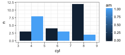
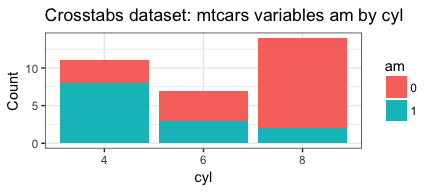
We originally started with a simple task using dplyr and ggplot2 in
the console. Take two of the mtcars variables, in this case am and
cyl, and conduct a cross tabulation and then plot it. Since it’s the
sort of thing I’m likely to do often seemed like a good candidate to
write a function for.
### with dplyr and ggplot manually
mtcars %>%
  filter(!is.na(am), !is.na(cyl))  %>%
  group_by(am,cyl) %>%
  count() %>%
  ggplot(aes(fill=am, y=n, x=cyl)) +
    geom_bar(position="dodge", stat="identity")
By the end of the last post we had accomplished the following tasks:
- Our function (called
PlotMe) was a lot more robust. It checked for basic user entry errors, added a useful plot title and generally did what we wanted. - Along the way we learned the “tricks” of working with
dplyrandggplot2inside of functions. - It allowed the user to choose the plot type from among three options
- We could feed it a pair of bare variable names e.g.
am&vsor through a helper we could also feed it multiple column numbers from the data frame and it would produce plots of all the combinations.
Here’s the PlotMeX function as we left it (with error checking removed
for clarity). If you’re not familiar with enquo or the !! notation
please refer back to an earlier post
here.
PlotMeX <- function(dataframe, x, y, plottype = "side"){
switch(plottype,
side = list(geom_bar(position="dodge", stat="identity"),
ylab("Count")) -> whichbar,
stack = list(geom_bar(stat="identity"),
ylab("Count")) -> whichbar,
percent = list(geom_bar(stat="identity", position="fill"),
ylab("Percent")) -> whichbar
)
aaa <- enquo(x)
bbb <- enquo(y)
dfname <- enquo(dataframe)
dataframe %>%
filter(!is.na(!! aaa), !is.na(!! bbb)) %>%
mutate(!!quo_name(aaa) := factor(!!aaa), !!quo_name(bbb) := factor(!!bbb)) %>%
group_by(!! aaa,!! bbb) %>%
count() %>%
ggplot(aes_(fill=aaa, y=~n, x=bbb)) +
whichbar +
ggtitle(bquote("Crosstabs"*.(dfname)*.(aaa)~"by"*.(bbb))) -> p
plot(p)
}
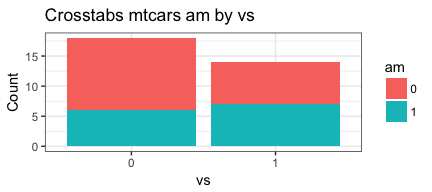
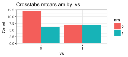
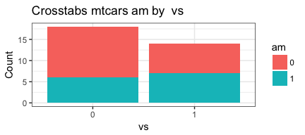
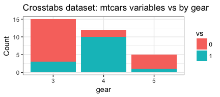
PlotMeX(mtcars, am, vs, "stack")
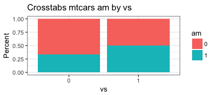
PlotMeX(mtcars, am, vs, "percent")
PlotMeX(esoph, alcgp, tobgp, "side")
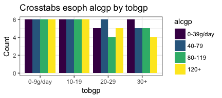
As you can see it works fine as far as we can tell on the mtcars data
set as well as the esoph dataset (which is also smallish). The problem
I discovered was that it was gross in performing on bigger datasets.
Especially if I fed it to mapply. Made no sense since I was not
plotting a full dataset I was plotting the crosstab data which is
already summarized and doesn’t have a lot of rows or columns. Something
was wrong.
What went wrong
Turns out I made two mistakes. Both of them had to do with how much data
I was accumulating especially over larger data sets or over repetitions.
3 keys tools may help you figure these things out. microbenchmark,
benchplot and just good old fashioned inspection of what the results
the function returns are.
# deliberately surpressing the figures!
microbenchmark(PlotMeX(mtcars, am, cyl), times = 10)
## Unit: milliseconds
##                      expr      min       lq     mean   median       uq
##  PlotMeX(mtcars, am, cyl) 244.5679 254.0199 255.1998 256.5568 257.5296
##       max neval
##  262.8945    10
benchplot(mtcars %>%
  filter(!is.na(am), !is.na(cyl))  %>%
  group_by(am,cyl) %>%
  count() %>%
  ggplot(aes(fill=am, y=n, x=cyl)) +
    geom_bar(position="dodge", stat="identity"))
##        step user.self sys.self elapsed
## 1 construct     0.005    0.000   0.005
## 2     build     0.019    0.000   0.020
## 3    render     0.150    0.003   0.157
## 4      draw     0.065    0.009   0.095
## 5     TOTAL     0.239    0.012   0.277
# don't forget to check your "returns"
inspectthisobject <- PlotMeX(mtcars, am, cyl)
In my case I decided to play it extra safe and add a intermediate
dataframe called tempdf. That way it would be much harder to ever
accidentally return too much data no matter how I called or invoked the
function.
    count() -> tempdf
  tempdf %>%
But the real culprit was dfname <- enquo(dataframe) which should have
been dfname <- deparse(substitute(dataframe)) or you run the risk of
passing back way too much data within the subsequent
ggtitle(bquote("Crosstabs"*.(dfname)*.(aaa)~"by"*.(bbb))).
Okay, now our PlotMeX has become…
PlotMeX <- function(dataframe, x, y, plottype = "side"){
switch(plottype,
side = list(geom_bar(position="dodge", stat="identity"),
ylab("Count")) -> whichbar,
stack = list(geom_bar(stat="identity"),
ylab("Count")) -> whichbar,
percent = list(geom_bar(stat="identity", position="fill"),
ylab("Percent")) -> whichbar
)
aaa <- enquo(x)
bbb <- enquo(y)
xname <- deparse(substitute(x))
yname <- deparse(substitute(y))
dfname <- deparse(substitute(dataframe))
dataframe %>%
filter(!is.na(!! aaa), !is.na(!! bbb)) %>%
mutate(!!quo_name(aaa) := factor(!!aaa), !!quo_name(bbb) := factor(!!bbb)) %>%
group_by(!! aaa,!! bbb) %>%
count() -> tempdf
tempdf %>%
ggplot(aes_(fill=aaa, y=~n, x=bbb)) +
whichbar +
ggtitle(bquote("Crosstabs "*.(dfname)~.(xname)~"by "~.(yname))) -> p
plot(p)
return(dfname)
}
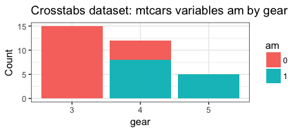
PlotMeX(mtcars,am,vs)
## [1] "mtcars"
PlotMeX(mtcars,am,vs, "stack")
## [1] "mtcars"
PlotMeX(mtcars,am,vs, "percent")

## [1] "mtcars"
That’s better. To summarize we now have PlotMeX which does our
plotting, the CrossXYs function which generates lists of things to be
plotted, and our error-checking code for user input that I have been
ignoring for awhile now. To remind you here’s CrossXYs.
CrossXYs <- function(dataframe, xwhich, ywhich){
  # Build two vectors
indvars<-list() # create empty list to add to
depvars<-list() # create empty list to add to
totalcombos <- 1 # keep track of where we are
message("Creating the variable pairings...")
for (j in seq_along(xwhich)) {
  for (k in seq_along(ywhich)) {
    depvars[[totalcombos]] <- as.name(colnames(dataframe[xwhich[[j]]]))
    indvars[[totalcombos]] <- as.name(colnames(dataframe[ywhich[[k]]]))
    cat("Pairing #", totalcombos, " ", as.name(colnames(dataframe[xwhich[[j]]])),
        " with ", as.name(colnames(dataframe[ywhich[[k]]])), "\n", sep = "")
    totalcombos <- totalcombos +1
  }
}
return(invisible(list(depvars=depvars,indvars=indvars)))
}
CrossXYs(mtcars,c(10:11),c(2,9))
## Creating the variable pairings...

## Pairing #1 gear with cyl
## Pairing #2 gear with am
## Pairing #3 carb with cyl
## Pairing #4 carb with am
Consolidate for success
My original plan had been to leave them as separate functions and use
mapply to invoke a multiplot option. But the more I thought about it
the more I liked the idea of one function that took care of everything.
So what I needed to do was combine the two and figure out from what the
user supplies which path to pursue. Here’s the finished product. For now
(as we troubleshoot) I have programmed it to return the arguments it was
passed. If you want to refresh your memory on the error checking pieces
please refer to this post.
PlotMeX <- function(dataframe, xwhich, ywhich, plottype = "side"){
  # error checking
  if (!require(ggplot2)) {
    stop("Can't continue can't load ggplot2")
  }
  theme_set(theme_bw())
  if (!require(dplyr)) {
    stop("Can't continue can't load dplyr")
  }
  if (length(match.call()) <= 3) {
    stop("Not enough arguments passed... requires a dataframe, plus at least two variables")
  }
  argList <-  as.list(match.call()[-1])
  if (!exists(deparse(substitute(dataframe)))) {
    stop("The first object in your list does not exist. It should be a dataframe")
  }
  if (!is(dataframe, "data.frame")) {
    stop("The first name you passed does not appear to be a data frame")
  }
  switch(plottype,
         side =  list(geom_bar(position="dodge", stat="identity"),
                      ylab("Count")) -> whichbar,
         stack = list(geom_bar(stat="identity"),
                      ylab("Count")) -> whichbar,
         percent = list(geom_bar(stat="identity", position="fill"),
                        ylab("Percent")) -> whichbar
  )
  # If both variables are found in the dataframe immediately print the plot
  if (deparse(substitute(xwhich)) %in% names(dataframe) & deparse(substitute(ywhich)) %in% names(dataframe)) {
    aaa <- enquo(xwhich)
    bbb <- enquo(ywhich)
    xname <- deparse(substitute(xwhich))
    yname <- deparse(substitute(ywhich))
    dfname <- deparse(substitute(dataframe))
    dataframe %>%
      filter(!is.na(!! aaa), !is.na(!! bbb))  %>%
      mutate(!!quo_name(aaa) := factor(!!aaa), !!quo_name(bbb) := factor(!!bbb)) %>%
      group_by(!! aaa,!! bbb) %>%
      count() -> tempdf
    tempdf %>%
      ggplot(aes_(fill=aaa, y=~n, x=bbb)) +
      whichbar +
      ggtitle(bquote("Crosstabs dataset: "*.(dfname)*" variables "*.(xname)~"by "*.(yname))) -> p
    return(p)
  }
  # If the user has given us integers indicating the column numbers rather than bare variable names
  # we need to build a list of what is to be plotted and then do the plotting
  # Build two lists
  indvars<-list() # create empty list to add to
  depvars<-list() # create empty list to add to
  totalcombos <- 1 # keep track of where we are
  message("Creating the variable pairings...")
  for (j in seq_along(xwhich)) {
    for (k in seq_along(ywhich)) {
      depvarsbare <- as.name(colnames(dataframe[xwhich[[j]]]))
      indvarsbare <- as.name(colnames(dataframe[ywhich[[k]]]))
      cat("Pairing #", totalcombos, " ", as.name(colnames(dataframe[xwhich[[j]]])),
          " with ", as.name(colnames(dataframe[ywhich[[k]]])), "\n", sep = "")
      aaa <- enquo(depvarsbare)
      bbb <- enquo(indvarsbare)
      xname <- deparse(substitute(depvarsbare))
      yname <- deparse(substitute(indvarsbare))
      dfname <- deparse(substitute(dataframe))
      dataframe %>%
        filter(!is.na(!! aaa), !is.na(!! bbb))  %>%
        mutate(!!quo_name(aaa) := factor(!!aaa), !!quo_name(bbb) := factor(!!bbb)) %>%
        group_by(!! aaa,!! bbb) %>%
        count() -> tempdf
      tempdf %>%
        ggplot(aes_(fill=aaa, y=~n, x=bbb)) +
        whichbar +
        ggtitle(bquote("Crosstabs dataset: "*.(dfname)*" variables "*.(xname)~"by "*.(yname))) -> p
      print(p)
      totalcombos <- totalcombos +1
    }
  }
  return(argList)
}
It’s a bit ugly and we need to clean it up, but it works whether the user gives me two bare variable names, or two sets of variables, or even just two column numbers
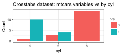
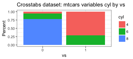
PlotMeX(mtcars, vs, cyl)
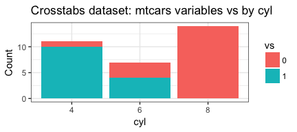
PlotMeX(mtcars, c(8:9), c(2,10), plottype = "stack")
## Creating the variable pairings...

## Pairing #1 vs with cyl
## Pairing #2 vs with gear
## Pairing #3 am with cyl
## Pairing #4 am with gear
## $dataframe
## mtcars
##
## $xwhich
## c(8:9)
##
## $ywhich
## c(2, 10)
##
## $plottype
## [1] "stack"
PlotMeX(mtcars, 2, 8, "percent")
## Creating the variable pairings...

## Pairing #1 cyl with vs
## $dataframe
## mtcars
##
## $xwhich
## [1] 2
##
## $ywhich
## [1] 8
##
## $plottype
## [1] "percent"
For those of you who have followed his whole series of posts you’ll notice that most of what is now in the function you have seen before. It’s just reorganized. We only handle the two “clean” cases of user input all bare variables or all integers. The key differences I would note are:
  # capture the arguments we're passed in
  argList <-  as.list(match.call()[-1])
  # An if test to see if both variables are bare
  # if they are we'll execute immediately
  if (deparse(substitute(xwhich)) %in% names(dataframe) & deparse(substitute(ywhich)) %in% names(dataframe))
  # these two commands move us from column number inside the loop to bare variable name
  depvarsbare <- as.name(colnames(dataframe[xwhich[[j]]]))
  indvarsbare <- as.name(colnames(dataframe[ywhich[[k]]]))
Performance wise, let’s rerun the same microbench as earlier. The
original mean time was ~255 milliseconds.
# deliberately surpressing the figures!
microbenchmark(PlotMeX(mtcars, am, cyl), times = 10)
## Unit: milliseconds
##                      expr      min       lq     mean   median       uq
##  PlotMeX(mtcars, am, cyl) 9.073721 9.444969 10.52728 9.970719 10.86919
##       max neval
##  14.90618    10
Our new benchmark? About 9 milliseconds! Very nice! We seem to have
accomplished what we set out to do. Just to be safe I also tested
against the much larger (N=51020) happy dataset from the
productplots package it took ~18 milliseconds.
All done (not yet!)
This has become a very long post so I’m going to end here. Next post we’ll cleanup our code and try and address some likely issues.
I hope you’ve found this useful. I am always open to comments, corrections and suggestions.
Chuck (ibecav at gmail dot com)
License

This
work is licensed under a
Creative
Commons Attribution-ShareAlike 4.0 International License.